ANDROMEDA-SHOCK (or, how to intepret HR 0.76, 95% CI 0.55-1.02, p=0.06)

[ADAlthousePhD]

However, they must be designed and implemented well if a result worthy of generalization to clinical practice is desired. An RCT that is so under powered that a quite large reduction in death (8.5% absolute difference in death at 28 days!) is not statistically significant is a major design flaw.

Agreed, with one caveat: given that this trial was entirely unfunded, run on the goodwill of the participating physicians and centers alone - I am inclined to go easy on the ANDROMEDA-SHOCK trialists for this. Yes, it’s a design flaw, and one of the trial investigators who spoke to me on Twitter admitted as much, but this trial seems to have some value as-is (this isn’t a drug/device approval on the line, but probably suggestive that at a bare minimum capillary refill time is an acceptable alternative to lactate monitoring where lactate monitoring is not available).

But I fully agree with this:

It’s important to publish both positive and negative trials, but it is also important to not take flawed “negative” trials and present them with unwavering, overly rigid interpretations of potentially strong signals. The formulaic interpretation of: RCTs infallible, p>0.05 means intervention useless is deeply flawed.

The rote use of phrases like “did not reduce…” and “no significant difference” is extremely frustrating, and something that journals should do better with.

[venkmurthy]

I don’t disagree, but I wasn’t aware that top journals gave extra credit for running a trial on too few resources rather than the clinical implications of the study (that is unless the use of fewer resources is itself innovative, e.g. registry RCTs).

Here they elevate a trial which deserves credit but is no more than hypothesis generating in its results (as analyzed). In doing so, they subject it to a false rigor in interpretation/reporting that were developed for trials with designs and power sufficient to be definitive.

[kiwiskiNZ]

The rote use of phrases like “did not reduce…” and “no significant difference” is extremely frustrating, and something that journals should do better with.

I’ve enjoyed scrolling through this discussion. I share Andrew’s frustration. When I first “got into” trials I did not find it easy (& sometimes still don’t) to find accurate alternative wording. My preference is to let the numbers speak for them selves and simply say “the difference was X (CI…)” or the “change was …” . But others may have better ways at expressing these things - I’d love to hear them? In particular, I’m interested in how to express a result when, for example, lower bound of the CI is more important than the point estimate?

[chrisarg]

Expensive invasive test vs something you can do by yourself , establishing rapport and actually justifying your clinical salary.

So yes the study killed the lactate even if one wanted to state no difference based on p=0.06

Nothing to discuss - no lactate for you

[HalilMD]

https://twitter.com/ihtanboga/status/1097566364821270529

Agree with @chrisarg that capillary refill method is easier and cheaper than lactat measurement. So, whether you use frequentist or bayesian methods, capillary refill wins.
@ADAlthousePhD: I calculated amateurly bayesian stat. using study results and used Kaul&Diamond paper/Calc and Wijeysundera paper for calc.
@f2harrell or @Anupam_singh may help for detailed code.

[DanLane911]

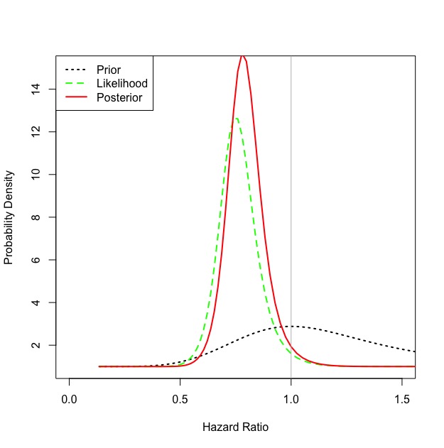
I estimated the Bayesian posterior using a skeptical prior (mean no effect, standard deviation extending 5% past MCID) and methods proposed in this paper. As you suggested the probability of HR<1 was 0.95, with a HR of 0.78 95% Certainty Interval 0.59-1.04.

I’d argue this is strong evidence for adopting the capillary refill time as the target end-point, instead of the more invasive and less direct measure of tissue hypoperfusion given by lactate.

Limitation: This method assumes normal distributions of the parameters.

R Code (Please point out if there are any errors so I can use again)
*Update: Code has been refined with help from @BenYAndrew
#Calculating MCID#

#Here I am using the estimated reductions from the power calculation to get an OR for the MCID (may need to be converted to RR instead of OR)#
n < - 420 #Sample size
a <- 0.3 * n #Intervention and Outcome
b <- 0.45 * n #Control and Outcome
c <- n - a #Intervention No Outcome
d <- n - b #Control No Outcome

MCID <- ((a+0.5) * (d+0.5))/((b+0.5) * (c+0.5))

#Hazard Ratio

HR <- 0.75
UCI <- 1.02

#Calculate Prior
#Skeptical prior mean estimate
#Calculating skeptical prior SD estimate for 5% probability of exceeding projected estimate
z <- qnorm(0.05)
prior.theta <- log(1)
prior.sd <- (log(MCID)-prior.theta)/z
#Enthusiastic Prior
prior.theta <- log(MCID)
prior.sd <- (log(1.05)-log(MCID))/qnorm(0.975)

#Calculate Likelihood
L.theta <- log(HR)
L.sd <- (log(UCI)-log(HR))/qnorm(0.975)

#Calculate Posterior
post.theta <- ((prior.theta/prior.sd^2)+(L.theta/L.sd^2))/((1/prior.sd^2)+(1/L.sd^2))
post.sd <- sqrt(1/((1/prior.sd^2)+(1/L.sd^2)))

#Calculate posterior median effect and 95% certainty interval
cbind(exp(qnorm(0.025, post.theta,post.sd, lower.tail = T)), exp(qnorm(0.5, post.theta,post.sd)), exp(qnorm(0.975, post.theta,post.sd)))

#Calculate probability benefit (HR < 1.0)
pnorm(log(1), post.theta,post.sd, lower.tail=T)

# Plot the prior density
mu.plot <- seq(-2,2,by=0.025)
prior <- dnorm(mu.plot, prior.theta, prior.sd)
likelihood <- dnorm(mu.plot, L.theta, L.sd)
posterior <- dnorm(mu.plot, post.theta, post.sd)

plot(exp(mu.plot), exp(prior),
type=“l”, col=“black”, lty=3,
xlim=c(0,1.5),
ylim=c(1,15),
lwd=2,
xlab=“Hazard Ratio”,
ylab=“Probability Density”)
#likelihood
lines(exp(mu.plot), exp(likelihood), col=“green”,lwd=2,lty = 2)
#posterior
lines(exp(mu.plot), exp(posterior), col=“red”,lwd=2)
abline(v=1, col = “gray”)

legend(“topleft”,
col=c(“black”,“green”,“red”),
lty=c(3,2,1),
lwd=2, #line width = 2
legend=c(“Prior”, “Likelihood”, “Posterior”))

[DanLane911]

Great minds think alike?

Dan Lane (DanLane911)

[ADAlthousePhD]

R Code (Please point out if there are any errors so I can use again)

Dan, thank you SO much for sharing this.

I think this is a huge potential of this site to improve knowledge. I will take a look thru this code tomorrow & Wednesday when I have some time. I know @f2harrell has been busy of late but if he can chime in as well that would be marvelous.

[f2harrell]

What @DanLane911 did is fabulous!

[Pavlos_Msaouel]

This is outstanding. Thank you so much for sharing this code! Only minor typo is there is a “UCI” instead of “UC” in the code that calculates the likelihood SD, which should be:

L.sd <- (log(UC)-log(HR))/1.96

[BenYAndrew]

Here is a quick and simple interactive adaptation of @DanLane911’s awesome code using Shiny: https://benjamin-andrew.shinyapps.io/andromeda_shock_bayesian/. The top right of the plot displays: (1) posterior probability of HR < 1 and (2) the prior probability ‘above’ the MCID (i.e., HR < 0.524) as a measure of prior skepticism. Would probably benefit from some more flexibility in defining the prior (i.e., ability to manipulate the % of prior above MCID directly), which I’ll work on. Happy to include anything else that may be useful and, of course, welcome any criticisms/comments/revisions! Code is here: https://github.com/andrew10043/andromeda_shock_bayesian/blob/master/app.R.

[ADAlthousePhD]

Incredible, @BenYAndrew and @DanLane911. I have a busy day today but tomorrow is fairly free and I cannot wait to start working with this, and it’s incredible that you shared this so we can have a good crowd-sourced discussion of the ANDROMEDA-SHOCK results with a variety of approaches. Cheers!

[f2harrell]

@BenYAndrew one suggestion is to allow the user to specify either the cutoff and the probability of exceeding it (or being less than it) or the SD. The former would result in the computed SD being displayed as text by the plot. Here is one suggested phrasing, keeping in mind that it’s not always the MCID that one wants to use.

Cutoff for HR for computing the width of the prior distribution (e.g., MCID): _____
Probability that the HR is less than this cutoff, or that 1/HR exceeds 1/cutoff: _____
or
Standard deviation of the prior distribution for the log hazard ratio: _____

[Gus_Hamilton]

This is absolutely fantastic. As an infectious disease physician, and a long time lurker and someone with a minimal (but growing) understanding of Bayesian statistics, this interpretation seems to me to be much more intuitive than the current reporting of the trial, and clearly represents a step forward.

@BenYAndrew - this is really fantastic. I am teaching the medical students this afternoon and will show them this!

Thanks
Fergus Hamilton
SpR Infectious Diseases, Bristol Royal Infirmary, UK

[BenYAndrew]

The app is updated to reflect some of @f2harrell’s suggestions. Right now the plot will only respond to changes in the prior SD slider bar, but I’m working on updating such that the probability bar will function as well.

[BenYAndrew]

This functionality should be working now. There are still some funky changes that may happen as you reach the extremes of various sliders that I’ll work out in the near future.

[alenghat]

I’m new to this platform; this is great. Here to provide a clinical perspective in this case. Has anyone spotted any report in the paper of differences in time spent with patient? I couldn’t find it. Each CRT measurement will require that someone (apparently ICU MD according to the method) is at bedside, and the CRT was performed four times more frequently (every 30 mins) than the lactate measurement (every 2 hrs, which requires no physician at bedside). So CRT is easier only in the sense that it does not involve a blood draw, but it is more intense in that it forces a physician to interact with the patient (and therefore, also with the ICU nurse caring for the patient) more frequently, which I’d like to think is still a good thing. I think that matters.

[BenYAndrew]

If the shinyapps.io page is non-responsive (only allows a certain level of traffic), you can alternatively view the application locally (if you have R and Shiny installed on your machine) by typing: runGitHub( “andromeda_shock_bayesian”, “andrew10043”)

[Anders_Perner]

Dear colleagues. Baysian or not, a major problem is that point estimates of small trials are unstable and may even change the direction with more pts enrolled. We have limited data from critical care trials, but I would be more comfortable to drop lactate if a 1000 pts had been enrolled

[ADAlthousePhD]

That’s an excellent point, Anders. I agree that the trial would provide more precise estimate if it had been larger, and that simply “switching to Bayes” does not fix that on its own. However, the rigid NHST interpretation of “cap refill time does not reduce mortality vs lactate” (because p>0.05) is not a very accurate description of the results; the Bayesian statements can say that “given the data observed in the trial, there is a fairly high probability that a strategy guided by capillary refill time is equal or better than lactate.”

The noisy point estimate could indeed drift back towards 1 with more data collection; the Bayesian posterior probability that the effect favors is our hedge against this, by telling us how likely it is that CRT has a net positive effect given the data observed thus far (Bayesian experts: help me refine this if I’ve stated something incorrectly).