My approach is maybe a bit convoluted by just doing all the backcomputation, so hopefully someone can add something better below if they find it. But you could to this.
Recall the definition of the OR:
((Number of cases with exposure)/(Number of cases without exposure)) / ((Number of non-cases with exposure)/(Number of non-cases without exposure))
I’ll assume here sex is the exposure, so you would divide:
((Infected men) / (Infected women)) / ((Non-infected men) / (Non-infected women))
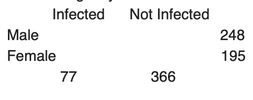
|
Infected |
Not infected |
Totals |
| Male |
A |
B |
248 |
| Female |
C |
D |
195 |
| Totals |
77 |
366 |
443 |
OR = 1.1 = (A/C) / (B/D)
C = 77 - A (because A + C = 77)
B = 248 - A (because A + B = 248)
D = 195 - C (because C + D = 195)
D = 195 - (77 - A) = 118 + A (replace C with 77 - A)
OR = 1.1 = (A / (77-A) / ((248-A) / (118 + A))
Solving this last bit you can do in R. You know the potential range for A is 0 to 77 (no exposed case to all cases are exposed). So you simply create a vector x with this range of numbers and then feed these into the formula:
> x <- seq(1,77,1)
> or <- (x/(77-x)) / ((248-x)/(118+x))
> or
[1]  0.006339229  0.013008130  0.020022063  0.027397260  0.035150892  0.043301129  0.051867220  0.060869565
[9]  0.070329806  0.080270914  0.090717300  0.101694915  0.113231383  0.125356125  0.138100512  0.151498021
[17]  0.165584416  0.180397937  0.195979521  0.212373038  0.229625551  0.247787611  0.266913580  0.287061995
[25]  0.308295964  0.330683625  0.354298643  0.379220779  0.405536530  0.433339840  0.462732919  0.493827160
[33]  0.526744186  0.561617040  0.598591549  0.637827888  0.679502370  0.723809524  0.770964493  0.821205821
[41]  0.874798712  0.932038835  0.993256815  1.058823529  1.129156404  1.204726924  1.286069652  1.373793103
[49]  1.468592965  1.571268238  1.682741117  1.804081633  1.936538462  2.081577768  2.240932642  2.416666667
[57]  2.611256545  2.827700831  3.069664903  3.341677096  3.649398396  4.000000000  4.402702703  4.869565217
[65]  5.416666667  6.065934066  6.848066298  7.807407407  9.010474860 10.561797753 12.635593220 15.545454545
[73] 19.918571429 27.218390805 41.835260116 85.720930233          Inf
> which(abs(or-1.1)==min(abs(or-1.1)))
[1] 45
So the number of exposed cases (A) is approximately 45.
You can automate this procedure if you keep in mind the following:
|
Outcome+ |
Outcome- |
Totals |
| Exposure+ |
A |
B |
Gamma |
| Exposure- |
C |
D |
Delta |
| Totals |
Alpha |
Beta |
Alpha + Beta |
Alpha = total individuals with the outcome (cases)
Beta = total individuals without the outcome (non-cases)
Gamma = total exposed individuals
Delta = total unexposed individuals
C = Alpha - A
B = Gamma - A
D = Delta - C = Delta - (Alpha - A) = Delta - Alpha + A
The following R function solves any 2x2 table similar to the method showcased above:
crosstable_components <- function(ncases,ncontrols,nexposed,nunexposed,or){
  referenceOR <- or
  x <- seq(1,ncases,1)
  b <- nexposed
  c <- ncases
  d <- nunexposed - ncases
  total <- ncases + ncontrols

  sequenceOR <- (x/(c-x)) / ((b-x)/(d+x))

  index_closestOR <- which(abs(sequenceOR-referenceOR)==min(abs(sequenceOR-referenceOR)))
  closestOR <- sequenceOR[index_closestOR]

  out_exposedcases <- round(index_closestOR,0)
  out_nonexposedcases <- round(c - out_exposedcases,0)
  out_exposednoncases <- round(b - out_exposedcases,0)
  out_nonexposednoncases <- round(d + out_exposedcases,0)

  filled_table <- matrix(data = c(out_exposedcases,out_nonexposedcases,ncases,
                                  out_exposednoncases,out_nonexposednoncases,ncontrols,
                                  nexposed,nunexposed,total,
                                  closestOR,NA,NA),
                         nrow = 3, ncol = 4)
  colnames(filled_table) <- c("Cases","Controls","Total","Closest Matched OR")
  rownames(filled_table) <- c("Exposed","Unexposed","Total")
  return(filled_table)
}
Edit: COOLSerdash was quicker and his answer is basically the same approach. Note that just like in his example where the issue comes down to rounding, in the method I use you are also faced with how precise the OR that you use as a reference is. In this case, two potential values of A (44 and 45) both round to 1.1, but the one with A = 45 is a bit close: 1.13 versus 1.06. Both my approach and the one from @COOLSERDASH will give approximations that are limited by the precision of the reporting of the studies you examine.