Frank, a part of your response I don’t understand is the rationale for using R^2, by which I presume you mean the squared correlation of the observed and fitted outcomes (if not, what are you using it for?). Hence I must ask you to please explain why and how you are using R^2; after all, there is a fair bit of literature on its scaling defects as well as its detachment from contextually relevant measures of effect, model fit, and predictive loss, e.g., Cox DR, Wermuth N, A comment on the coefficient of determination for binary responses. Am Statist 1992;46:1–4. Rosenthal RB, Rubin DR, A note on percent variance explained as a measure of importance of effects, J Appl Soc Psychol 1979;9:395–396. Greenland S, Schlesselman JJ, Criqui MH, The fallacy of employing standardized regression coefficients and correlations as measures of effect. Am J Epidemiol 1986;123:203–208. Greenland S, A lower bound for the correlation of exponentiated bivariate normal pairs. Am Statist 1996;50:163–164.
Hi Sander - I was referring to the deviance-based R^2 measures listed here. My favorite one uses the effective sample size and penalizes for the number of parameters in a very similar way that ordinary linear model R^{2}_\text{adj} does.
Thanks Frank for the explanation. The measures you cite can be viewed as generalizations of the original Gaussian R^2 I mentioned, and inherit all of the original R^2 scaling defects as well as detachment from contextually relevant measures of effect, model fit, and predictive loss.
Those defects have not stopped me (or anyone I know) from looking at such measures as part of a suite of model diagnostics; and the adjustments your article mentions (such as penalization against overfitting) are definite improvements. Even if used alone the measures are better than no check at all (which I think is the norm in the research literature I see). But presumably you would agree that, if the purpose of the model is to come up with reliable individual predictions for clinical decisions (as opposed to just estimating associations or effects averaged over the data source), much more detailed and contextually relevant checks are needed.
Yes, agree with all. I use generalized R^2 indexes primarily as measures of predictive discrimination / predictive information and not as goodness-of-fit measures.
Okay @Pavlos_Msaouel, in keeping with your impressive efforts to translate challenging statistical concepts into clinician-speak (e.g., statements like: “When a model that allows for treatment effect homogeneity finds effect heterogeneity, I come close to believing it”), here’s a summary of my current understanding based on your publications. The statistics literature is unbelievably convoluted in its explanations of interaction, so it’s no surprise that clinicians get confused. Others can advise whether this Unabomber Manifesto is either overly simplistic or just plain incorrect…
Statistical interactions that are observed in RCTs need to be interpreted with extreme caution in order to avoid drawing the wrong conclusions and making unsound recommendations to patients.
Observed statistical interaction (where the relative treatment effect observed within a subgroup differs from the relative treatment effect in the overall trial population) can be a function of 1) biologic heterogeneity i.e., differing underlying biologic capacity to respond to the treatment within certain trial subgroups; or 2) prognostic heterogeneity within certain trial subgroups; or 3) low power.
Biologic heterogeneity
-
Biologic heterogeneity can potentially be the main driver for an observed subgroup-specific statistical interaction. This is the type of heterogeneity that is of greatest interest to researchers/clinicians in a trial. Identification of true biologic heterogeneity can advance our understanding of underlying disease mechanism and suggest potentially fruitful new lines of research;
-
However, biologic heterogeneity is generally not expected to occur very commonly within highly selected trial populations, since researchers have usually gone to great lengths to optimize the “biologic responsiveness” of the subjects they enrol in their trials. Since pre-clinical and early phase clinical research is typically extensive, disease mechanisms are often well understood by the time a drug reaches phase III;
-
Patient-level characteristics that confer true biologic heterogeneity are known as “predictive” factors (e.g., the presence of a certain receptor on a patent’s lung tumour that confers responsiveness to a certain targeted therapy.)
Prognostic heterogeneity
-
Alternately, prognostic heterogeneity can potentially be the main driver for an observed subgroup-specific statistical interaction. Examples of covariates that might be prognostic in nature include patient age or baseline disease severity. For a subgroup defined by a prognostic covariate, any observed statistical interaction within the subgroup will reflect features of the patient that are related to his baseline prognosis, rather than any underlying differential biologic capacity for him to respond to the therapy (e.g., a unique feature of his particular tumour). In this scenario, the subgroup-specific statistical interaction is observed primarily because the covariate being used to define the subgroup is one that has simply rendered the signal of therapeutic efficacy easier to detect.
-
Signals of prognostic heterogeneity are not considered to be as valuable to detect during a trial as are signals of biologic heterogeneity, because signals of prognostic heterogeneity don’t generally advance our understanding of underlying biological mechanisms. As a result, such signals don’t generally help to inform future avenues of research;
-
Indeed, observed statistical interactions which stem from prognostic heterogeneity can be considered “nuisance” phenomena in the context of a trial since it can be challenging to differentiate predictive factors/covariates from prognostic factors/covariates;
-
Importantly, some patient-level covariates/factors can be BOTH predictive AND prognostic (e.g., HER2 receptor positivity of a patient’s breast cancer in a trial designed to test a therapy that targets the HER2 receptor);
-
Prognostic heterogeneity is an important consideration when designing a trial. Stratifying randomization according to prognostic factors and making a plan to adjust for them in the analysis phase of the trial can improve the power of a trial;
-
Individual patients’ prognoses will also influence the absolute benefit that they might reasonably expect to incur with treatment. The preferred way to incorporate such prognostic considerations in decision-making is at the point of care, after a trial is done;
-
Ideally (though far too infrequently), “risk calculators” will have been developed for the disease in question, using large, detailed observational datasets. These datasets will have permitted identification of important prognostic factors (e.g., age, baseline disease severity, presence/absence of certain comorbidities…). Clinicians enter these prognostic factors into a calculator at the point of care, generating an estimate of the patient’s future risk for experiencing the outcome of interest in the absence of treatment. Then, the relative treatment effect (as identified through an RCT) gets multiplied by the patient’s estimated baseline risk for experiencing the outcome. This generates an estimate of the absolute risk reduction that the patient might reasonably be expected to incur with treatment. He can then decide if this degree of benefit is “worth it” to him (depending on his own/personal value system).
Low power
-
Low power creates wide-ranging consequences for the interpretation of subgroup-specific statistical interactions observed in trials, quite aside from the challenges we face in differentiating predictive factors/covariates from prognostic factors/covariates;
-
Arguably, low power will always be the most fundamental consideration when trying to interpret statistical interactions observed within subgroups. If power is low, robust interpretation of observed statistical interactions is impossible. And this will ALWAYS be the case for subgroup analysis, since trials are sized/powered for assessing the relative treatment effect in the overall trial population, NOT for assessing the relative effect within subgroups;
-
Low power can result either in the trial’s inability to signal the presence of a true subgroup-specific effect OR in generation of a signal of a potential subgroup effect when no such effect actually exists;
Implications for approaching subgroup analysis in RCTs
-
It’s essential not to conflate the detectability (or not) of a therapeutic effect within certain patient subgroups with assessment of that subgroup’s biologic capacity to respond to the therapy. If clinicians do this, they could end up making poor decisions regarding the types of patients who get offered treatment after the trial is done;
-
We should always focus preferentially on a trial’s overall result, rather on subgroup findings;
-
If we see an encouraging relative therapeutic effect in the overall trial population but the effect seems diminished when analyzing a specific patient subgroup, we should generally NOT infer that the therapy “lacks efficacy” in that subgroup;
-
Conversely, in the face of a non-compelling (neutral) result for the overall trial population, “signals” of therapeutic efficacy that are confined to trial subgroups are highly likely to be false signals stemming from underpowering. This is because it’s very unlikely, given the rigour of the drug development gauntlet, that a drug reaching phase III would end up, “unexpectedly,” having beneficial effects in some subgroups but harmful effects in other subgroups AND that all of these various subgroup effects would just “happen” to offset each other so perfectly that the overall trial result would end up being neutral;
-
Whether a particular covariate is expected to be predictive or prognostic in nature should be defined in the design phase of an RCT, based on known biology and pre-trial information;
-
Since subgroup analyses will always be underpowered and therefore suboptimally robust, we should not allow them to influence, unduly, decisions around which patients to treat (or not treat) after the trial is done. For example, we should know enough to expect that a trial will be less likely to detect a treatment’s relative efficacy signal when we analyze the subgroup of patients with less severe baseline disease, as compared with the subgroup with more severe baseline disease. If we expect this finding, then later, when we observe this phenomenon while analyzing the trial’s results, we will recognize it for what it is- namely, a consequence of underpowering. Patients who are less sick at baseline will accrue fewer outcomes of interest during the trial, but this doesn’t mean that the drug isn’t, mechanistically, “doing what it’s supposed to do” within their bodies. Importantly, if we go into a trial expecting this prognostic phenomenon to occur, we will not be tempted to mistake it for a lack of biological capacity to respond within the subgroup defined by that prognostic covariate;
-
We should have even LESS faith than usual in the results of a subgroup analysis that was not prespecified (in the design phase of the trial, based on known biology), but rather conducted “post hoc” (as a data-dredging exercise);
-
If researchers have reason to suspect, based on lab experimentation, that a certain patient-level covariate might confer a differential biologic response to the therapy being tested, but if the trial accrued few outcomes of interest within this subgroup, then researchers’ prior hypothesis of a potential subgroup effect should not necessarily be discarded- absence of evidence is not evidence of absence;
-
Conversely, if researchers have NO reason to suspect, going into a trial, that a certain patient-level covariate might confer a differential biologic response to the therapy being tested, but if a statistical interaction is nonetheless observed within a certain subgroup during a post hoc analysis, then researchers will be left asking themselves whether the observed statistical interaction is reflecting predictive heterogeneity or prognostic heterogeneity, or NEITHER (i.e., the statistical interaction might simply represent a “spurious” heterogeneity signal stemming from underpowering). This is why post hoc subgroup analysis can end up being so misleading. Pursuing multiple statistical interaction signals that have a low a priori likelihood of reflecting true biologic heterogeneity can end up wasting a lot of money and harming patients;
-
Since 1) biologic heterogeneity (differential biologic capacity to respond) is not generally expected to be present (or to be present to a meaningful degree) within clinical trials of therapies with a well-understood mechanism of action (due to rigorous patient selection practices); and 2) signals of prognostic heterogeneity are not considered important to detect in the context of a trial and can just create inferential difficulties (i.e., difficulty distinguishing predictive factors from prognostic factors), trialists will generally prefer to use effect measures which are less “labile” (i.e., less likely to fluctuate) in response to prognostic heterogeneity;
-
True biologic interaction/effect modification will often have a dramatic effect on the relative treatment effect observed within a subgroup defined by presence of the interacting factor (provided that enough outcomes of interest have been accrued among subjects with the biologically-interacting characteristic). For example, if certain patients’ tumours lack the receptor through which a targeted cancer therapy is known to exert its effect, then we would expect NO efficacy to be demonstrated among patients whose tumours lack that receptor if those patients had been enrolled in a trial of that therapy. Arguably, however, we’d expect such patients to have been actively excluded from the trial based on detailed pre-trial knowledge of the drug’s mechanism of action;
-
Given rigorous patient selection protocols for trials involving therapies with well-understood mechanisms of action, true biologic interaction, if present in a trial, will likely be observed only very rarely and will invariably be viewed as an “unexpected”/serendipitous discovery. Attempts to understand the reason for the interaction could lead to a deeper understanding of disease mechanism and therefore to new treatments;
-
Competing imperatives to not fail to detect true biologic interactions while simultaneously not over-reacting to false signals of biologic interaction (i.e, those that might reflect either prognostic heterogeneity or simple underpowering), explains trialists’ preference for 1) subgroup analysis that is pre-specified and justified by biologic plausibility, and 2) effect measures that are more stable/less labile;
-
Trialists will prefer using effect measures that are less likely to generate signals of statistical interaction in situations when the type of statistical interaction they are most concerned about not missing (i.e., biologic interaction) is expected to be absent (e.g., in the context of a clinical trial with highly selected patients);
-
Trialists will prefer to use an effect measure that behaves in such a way that it will remain “responsive enough” to be perturbed in the presence of true biologic interaction, but not so responsive that it is vulnerable to perturbation by factors other than true biologic heterogeneity;
-
Whereas a subtle perturbation in the relative treatment effect, if observed within a particular subgroup, could reflect either underlying prognostic heterogeneity OR a signal of biologic/predictive heterogeneity that has been weakened by underpowering, OR simple underpowering alone, dramatic perturbation of the relative treatment effect within a subgroup is more likely to reflect true biologic interaction/effect modification.
-
It follows that if an effect measure that’s known (historically) to be relatively “stable” nonetheless appears perturbed in a subgroup analysis, we should pay it more heed than if we had been using a more “labile” effect measure (“When a model that allows for treatment effect homogeneity finds effect heterogeneity, I come close to believing it…”).
Agree with a lot of the above, but my view is simpler and starts first from the following causal assumptions. We can roughly break down what clinicians (or at least most clinical oncologists) are interested in two relationships:
- Prognostic effects (also known as “risk magnification”, “risk modeling”, “risk score analysis”, “effect measure modification”, “additive effect”, “main effect”, or “heterogeneity of effect”). In an RCT (no arrow towards treatment choice X) they correspond to the following DAG whereby X is the treatment choice, Y is the outcome of interest, and Z is a covariate (such as patient age) affecting the outcome Y but not the pathway that mediates the treatment effect from X:
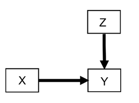
If we want to make decisions on how a treatment choice X influences the outcome Y for a specific patient, we do also need to know how Z also influences Y. This is the most common and high yield relationship to account for when thinking about outcome heterogeneity. We have written many methodology papers and trial designs focusing almost exclusively on this effect, e.g., here, here, here, here, and here. In extreme scenarios, if Z is very strongly influencing Y then it can effective nullify the choice of X. Say you have a patient with very aggressive cancer Z_1 that reduces median survival Y to 1 week. In this patient, the treatment choice X_1 between two drugs designed to optimize A1c in a timespan of years does not matter.
While prognostic effects via Z can effectively negate the treatment effect X on Y, they cannot flip its directionality to make it harmful for Y. However, notice that this applies only if we are focusing on one outcome Y (e.g., survival) that has the above causal relationship. If a patient’s prognostic covariates Z influence also outcomes such as specific deadly side effects aggravated by treatment choice X then directionality can be flipped. Thus, there is a whole lot of important things that “prognostic” effects influence.
- Predictive effects (also known in the literature as “effect modeling”, “treatment interaction”, or “multiplicative effect”). In an RCT (no arrow towards treatment choice X) they correspond to the following DAG whereby X is the treatment choice, Y is the outcome of interest, and B is a covariate affecting the pathway M that mediates the effect of X on Y:
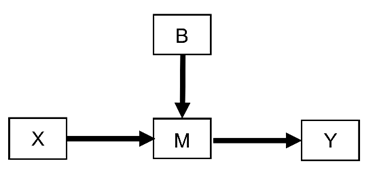
For example, B may be the presence or absence of cancer HER2 expression in an RCT testing the effects of cancer drugs X that target the HER2 pathway M to improve patient survival Y.
This is the scenario that in theory can more directly flip the directionality to make X harmful for Y. If HER2 is not expressed by a tumor then the effect of X will be zero. But the tumor may also express a pathway M_1 that actually feeds it when a treatment X_1 is given versus X_2 making the tumor grow faster when X_1 is used.
Thus, “prognostic” effects from Z tend to be more easy to model (including statistically) making them more high-yield for estimating treatment effect heterogeneity. Conversely, “predictive” effects from B to M and then to Y require more complex modeling but can have more profound negative implications (albeit more rarely) and are more relevant to drug design and preclinical research.
Note that I generally strongly dislike and discourage the use of the terms “prognostic” versus “predictive” to distinguish the above two scenarios but adopting them here because they are so heavily popularized (at least in oncology).
Thanks Pavlos! Great explanations as usual - a picture is worth a thousand words. I was trying to talk through (to myself) how a researcher’s focus on 1) not missing predictive factors that might show up (serendipitously) in an RCT while 2) guarding against misinterpreting other types of observed statistical interactions might explain a trialist’s preference for a certain effect measure (e.g., Odds Ratio).
Regarding the choice of effect measure these are the guiding principles I believe we should use:
- The primary analysis should use all the information in the raw data
- The primary analysis should use a model that is likely to fit the data
- Parameters in this model may be used for frequentist or Bayesian assessment of evidence for any treatment effect and will usually optimize power
- Model parameters should be transformed nonlinearly into a series of clinical readouts that clinicians will instantly connect with
- Generally speaking the evidence for any effectiveness based on these readouts will agree with the evidence for any effectiveness from the model parameters
- The two will not agree on the degree of clinical effects, and the transformed parameters giving the clinical readouts, and uncertainty intervals for them, should be used to judge degrees of effectiveness
For problems not using a linear model on a continuous outcome, primary model parameters that are associated with well-fitting models are typically parameters with unrestricted ranges such as log odds ratios (for standard effects or for state transitions) and log hazard ratios. Clinical readouts may include differences in outcome probabilities (absolute risk reduction), differences in cumulative incidence at a fixed time point or expected time in good states, each computed at covariate settings of interest. Absolute clinical effects cannot be averaged over covariates in a meaningful way, e.g., patients with more disease will have more movement in absolute quantities (unlike ORs, HRs, etc.).