I never thought a thread on the horoscope would be so interesting and productive. Thanks, let’s digest it.
2 Likes
In epidemiology and causality theory, horoscopes can be seen as an example of a negative control treatment - valuable precisely because everyone in the community will accept that they have no effect; hence an analysis making it look as if they do have an effect may be taken as a sign of a problem with the data or the analysis approach (or both).
4 Likes
This is true in so many aspects of statistics. To paint with only a slightly overly broad brush, much of mathematical statistics seems to be motivated by job preservation IMHO. I see so many one-off frequentist solutions to problems that could have been handled much more simply, but without getting a paper out of it. I’m thinking also of the field of large sample theory and asymptotics.
3 Likes
Yes indeed. I’ve heard similar comments from some top honored stat theory figures (one placed about 80% of what is published in Theory & Methods is like that). And a lot of it is reinventing wheels using new hubcaps. Of course top applied statisticians like you and Box have long complained about that. It seems to be a product of the perverse incentives for academic careers, where mathematical sophistication is mistaken for scientific sensibility and relevance. I think some of Sabine Hossenfelder’s complaints about theoretical physics are similar, e.g.,
On string theory: https://www.youtube.com/watch?v=6RQ6ugMWZ0c
On current cosmogony: https://www.youtube.com/watch?v=VHhUCav_Jrk
On many worlds: https://www.youtube.com/watch?v=kF6USB2I1iU
3 Likes
To be mentioned even on the same web site (not to mention the same page) as Box is quite an honor …
4 Likes
Well, I kept thinking about the problem.
I have calculated the day within the year in which the subject was born (Days_b, from 1 to 365), and I have divided it by 365 to obtain the fraction. I have learnt that the amplitude and phase of a sinusoidal function A * sin (x + phase) = a * sin (x) + b * sin (x), which helps to fit a regression equation (phase & amplitude may be solved from model coefficients). As a confounder I have added the year modeled in a non-linear way. The complete zodiac is problematic because it induces multicollinearity (VIFs >40).
Therefore, I followed @RonanConroy proposal and grouped them according to the four elements (water, fire, air, earth).
After that, no apparent seasonality, no prognostic effect associated with the zodiac (sorry!).
> fit<- coxph(Surv(time,event) ~ sin(2*pi*Day_S/365)+cos(2*pi*Day_S/365)+elements+rcs(year,3),data=data)
> fit
Call:
coxph(formula = Surv(time,event) ~ sin(2 * pi * Day_S/365) + cos(2 *
    pi * Day_S/365) + elements + rcs(year, 3), data = data)

                          coef   exp(coef)  se(coef)      z     p
sin(2 * pi * Day_S/365)  0.005699  1.005715  0.032472  0.176 0.861
cos(2 * pi * Day_S/365) -0.025517  0.974806  0.033196 -0.769 0.442
elementsEarth           -0.037949  0.962762  0.071303 -0.532 0.595
elementsFire            -0.070279  0.932134  0.073149 -0.961 0.337
elementsWater           -0.058129  0.943528  0.071917 -0.808 0.419
rcs(year, 3)year        -0.006045  0.993973  0.004463 -1.355 0.176
rcs(year, 3)year'        0.007015  1.007040  0.005497  1.276 0.202

Likelihood ratio test=3.95  on 7 df, p=0.7859
n= 2473, number of events= 2057
   (97 observations deleted due to missingness)
> vif(fit)
sin(2 * pi * Day_S/365) cos(2 * pi * Day_S/365)           elementsEarth            elementsFire           elementsWater
               1.083581                1.126406                2.049739                2.387306                1.985137
       rcs(year, 3)year       rcs(year, 3)year'
               5.978774                5.963942
What do you think? Mystery solved? Is this a good test as requested by prof @Sander ?
P.S. this may be overthinking the issue since the four elements alone are not either significant !
P.S… Do I need to explore >1 cycles per year?
3 Likes
[Typo: your first b * sin (x) should be b * cos(x)]
Yes a * sin (x) + b * cos(x) is an easier way to fit seasonality. Were this a serious analysis of seasonality you would then have to transform the stats for a and b into stats for amplitude A and phase. But no need for that here and your approach is better than what I suggested.
I can’t quite understand your model code: I missed what is rcs(year,3) and why is it in the model? What happens if you remove it?
Assuming that’s not an issue (and I think it’s not), your results are exactly like we all expected, and so I think your analysis is now a teaching demonstration of how initially seemingly odd results using what is in fact an odd overparameterized model (unordered months, inappropriate for examining either season or astrology) can evaporate or be explained away once one uses actual prior structural expectations; i.e., a model based on what the background context tells us what we ought to see IF there is any effect of these variables. With that, the model has now tried to be fair to both seasonal concerns and astrology. Hence I’d be most curious if anyone disagrees (even astrologers).
There is however one item I didn’t see that I’d want to see in any serious topic analysis: A test of model fit. If there is one available in your proc, perhaps you can run it just to show there is no obvious problem there. Again maybe this should be done without rcs (whatever that is) in the model.
3 Likes
rcs is restricted cubic spline also known as natural spline, using a truncated power basis. This is done by the R rms package. rcs(x, 3) means 3 default knots (points of discontinuity of the 3rd derivative) that have equal sample size between any two knots. With 3 knots rcs uses default knot placement, at the 0.05, 0.5, 0.95 quantiles of the predictor. This captures long-term time trends.
Thanks Frank, that clears up what the terms are but I’m still not following why rcs(year,3) in the model.
First, why is it used as opposed to say rcs(secular,3)? where “secular” is full calendar time running from 0 to end of study and increasing by 365 or 366 across each year (i.e., it’s not date within year). If “year” is literally just year then the model is implicitly forcing jumps at year boundaries, constraining them to follow an rcs across years only; but if the concern is to capture evolution of treatment and case mix, I’d expect neither to jump at Jan. 1 and nowhere else. Second, I would have expected any secular trend over a restricted period to be monotone, which the rcs does not enforce. So if the goal is simply to control confounding by secular trends I would have used up the two parameters (model df) for that quite differently. [Not that any of that matters in this example given the rcs coefficients are practically zero, so there appears to be no secular effect; but I’m treating it as a teaching example.]
Finally and most of all, I can’t see how “year” could be a confounder in this example because I expect the distribution of dates within each year to be practically constant across years, naturally preventing confounding of “date” by “year” and thus eliminating the need for “year” in the model even if (unlike here) it had some notable effect. One could even look at the data to check this independence prior (that being ancillary for the outcome regression, such a check does not invalidate the latter).
Am I missing something here?
1 Like
I am going step by step with this wonderful exercise.
The amplitude is equal to sqrt (coef1^2 + coef^2)
On the other hand, sin phase = coef2 / sqrt (coef1^2 + coef^2)
Therefore, if I do it correctly it would be:
> sqrt(0.005699^2 + (-0.025517)^2) # amplitude
[1] 0.02614567
> asin(-0.025517/( sqrt(0.005699^2 + (-0.025517)^2)))*365/(2*pi) # phase
[1] -78.48525
That is, a maximum of about day 365-78.4.
Seems right?
Although the phase has a simple interpretation, I am not sure how to interpret the amplitude. The tiny number I suppose is interpreted as little seasonality. However, we have to calculate the confidence interval to those quantities using the covariance matrix (maybe @RGNewcombe can help). I only know how to do this to add up the coefficients. I don’t know if any trick in R allows to do it.
With respect to rcs(year,3) it was to model the year of birth itself. In Spain some years were harder than others. In the years after the civil war there was a lot of misery. The conditions were slowly improving but then there have been several crises, etc.
Anyway, I find it very strange how easy it is to find these trends. For example, I have used a second database, and have repeated the analysis with or without seasonality and secular trends. It comes out the same as in the previous case. I have the feeling that there may be some weird mathematical artifact in the regression with a categorical variable with 12 levels. Maybe a simulation is a good idea as @zad suggested.
Fit 1: no seasonality, no secular trend
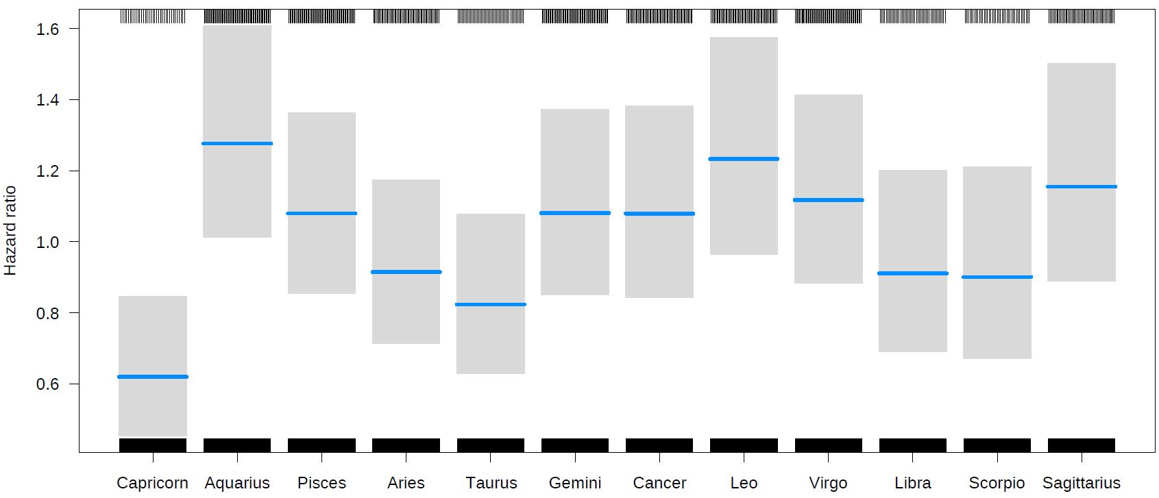
Fit 2. With seasonality and secular trend.

The result is quite impressive. I am going for the Cox diagnostics in a moment…
Great points Sander. Speaking generally this is my preferred approach:
- When the data span multiple years include a long-term time trend using a spline function of year + fraction of a year
- For cyclic within-year trends without assuming symmetry as sin and cos do, include an additional short-term trend in the model using cyclic splines
1 Like
How can in do that??
See http://www.mosismath.com/PeriodicSplines/PeriodicSplines.html
This is a fantastic resource on monotone splines (which doesn’t answer your question): https://rpubs.com/deleeuw/268327 .
2 Likes
Great resources indeed - thanks!
I have been reading these articles on s-values. I would like to be sure I understood it properly.
As I understand it, the p-value captures the probability of data under the null hypothesis. Thus, the p-value can be seen as the probability that the current sequence of information made up of the data is random, if H0 is true. The lower the p-value, the higher the number of micro-states from which the current sample could have been generated… This implies that our data are rarer under H0. For example, if the p-value = 0.0625, this implies that we have obtained this actual result from 1/2^4 possible random sequences. Since we know from Shanon that the information about these microstates grows exponentially, that is why -log2(p-value) is a measure of information in bits. Therefore, a p-value=0.0625 means that our data contains 4 bits against H0, which is not much, right?
Not sure of your question, but yes “p=0.0625 means that our data contains 4 bits against H0, which is not much” - at least, not much in the context of ordinary statistical research. There are other ways to formally measure the evidence and in particular see that p=0.0625 is “not much evidence” in these contexts, e.g., see the discussion of alternatives in sec. 4 of the supplement to Rafi-Greenland posted here: https://arxiv.org/pdf/2008.12991.pdf
4 Likes
The question was whether my understanding of the deeper meaning of s-values, based on Shanon’s theory, was correct. I think it is a beautiful concept and I would like to make it clear.
OK, I’ve looked again at your initial post today. First, I agree it is a beautiful theory - of course beauty does not mean it is useful for a given purpose, but I do think it is useful for understanding statistics.
I cannot however tell if you have grasped “the deeper meaning” of S-values, perhaps because I haven’t either; instead I see P-values and S-values as abstract math entities whose meaning remains to be assigned by any of a number of contextual-framework (semantic) overlays, depending on the story that gives rise to the test statistic and its distribution.
Also I am not clear about what you mean by your wording. You mention microstates in “The lower the p-value, the higher the number of micro-states from which the current sample could have been generated…”; however, as can be seen in a simple permutation test, the number of microstates (points in the sample/data space) that will produce the observed macrostate (the tail event of ‘T as or more extreme than t’, where t=observed test statistic) drops with p, dropping to just 1 in the most extreme case (as with all heads). So maybe you meant “The lower the P-value, the lower the number of microstates”? Or else I misunderstand something.
The rest looks OK to me; in particular yes the amount of information about the microstate grows exponentially as p declines - precisely because of the declining number of possible microstates giving the macrostate indexed by p.
Here is what I thought is a neat little PBS Digital show which may help you judge our grasp using statistical mechanics, allowing that the physics terminology differs from the stat/comm one we use -
In their terminology, entropy gauges the number of microstates that produce the macrostate, so small p means low entropy when the macrostate is the tail event:

For connections of statistical mechanics to statistical methods one place to start might be Jaynes - well worth reading on many grounds (just so long as you don’t become a dogmatic convert like some do); he died before completing it but it became a classic of sorts anyway: https://bayes.wustl.edu/etj/prob/book.pdf
Note how he must modify Shannon to deal rigorously with the continuous case (as everyone must).
3 Likes
I think the intuition for this abstract concept would be this:
Imagine that we have n categories of something, and we obtain random elements so that each observation has a 1/n probability. For example, we have 4 letters (A, B, C, and D), and the probability of each observation is 1/4. Then we can say that any single observation provides us -log2(1/4) bits of information (in this case 2 bits). This is so because the observation is equivalent to ask two binary questions. We can ask if it is AB vs CD, and depending on the answer we can then ask if it is A or C, so we have learned 2 bits. Similarly we can understand the p-value as the probability of the observed data under H0. Therefore, a p-value=1/4, gives us a learning of 2 bits of information against H0