Yes, that is correct. ![]()
There were past comments, not only here but debated elsewhere as well, on whether or not to include the baseline observation in the mixed effects model as a response, or only as a covariate.
I fall into the latter camp.
Yes, that is correct. ![]()
There were past comments, not only here but debated elsewhere as well, on whether or not to include the baseline observation in the mixed effects model as a response, or only as a covariate.
I fall into the latter camp.
The approach by Kurz seems overly simplistic to me, where there seems to be a narrow focus on the easy interpretation of the model coefficients, including the intercept term, at the expense of ensuring that you have the correct model to begin with. It also violates the principle of hierarchy, as was mentioned in prior comments by both Frank and me, where low order terms (main effects) should be in the model, if you are including high order terms.
When you create these models, you then generate post hoc, model based, marginal estimates of treatment effects, and that is typically done using the overall sample mean value as the baseline (pre-treatment) measurement, so that you get an estimate of the mean treatment effect over time.
In the setting of an RCT, the underlying question is, if we have two patients that start out with the same pre-treatment value (e.g. the overall sample mean), and we expose one patient to treatment A and the other patient to treatment B, all else being equal, what is the difference in the measurement at one or more relevant post-treatment time points?
That is the case whether you have a typical OLS ANCOVA model with a single pre and single post measurement, or in the context of a mixed effects ANCOVA type model, as discussed above, with a single pre measurement and multiple post measurements with subject level clustering.
There is no reason, in my mind, to constrain the model to some kind of parsimonious approach, simply for the sake of easy interpretation of coefficients, when you have the ability in statistical software, like R, to generate model based marginal estimates, and do so at varying values, or combinations of values, of the baseline covariates.
Importantly, you can take the same approach to estimate the marginal treatment effects, whether you have simple models, or very complex ones, with various transformations on the covariates.
What I find interesting, is that one of the references that Kurz lists on his web page, is the marginaleffects package by Vincent Arel-Bundock:
https://github.com/vincentarelbundock/marginaleffects
where the package author has the following content in his “Why?” section on that page:
The comment in the second sentence above (bolded) seems to be in conflict with Kurz’ expressed desire to have simple interpretations of the model coefficients as being the justification for leaving out the main effects of the treatment group.
The marginaleffects package seems to be conceptually similar to the emmeans package that I use, where the former is designed to use the ‘tidyverse’ framework, which I do not use myself. Both provide for a common interface to a large set of R models, across numerous packages, addressing the author’s last couple of sentences in the quote above.
HI Marc,
As always, thank you for your thoughtful and thought-provoking comments. Indeed, interpretative convenience should not come at the expense of model correctness, and your advice to fully specify a model and to estimate the model-based marginal effects using the emmeans or marginaleffects R packages is very well taken. That said, I was drawn to the blog post by Kurtz mainly because the multilevel ANCOVA conceptualization is reportedly able to handle missing values using full-information estimation. If true, this property may be useful in situations where study participants are missing on the follow-up outcomes.
Again, thank you for your advice and guidance.
@puayonghao, be aware that, while this is true for mixed effects models generally, when clustered observations are involved, not just in this pre/post setting with multiple post-treatment measurements, there is still an underlying assumption that the data, including baseline (pre-treatment) values, are missing at random to minimize bias.
The mixed effects analysis, in the absence of imputation, will still be performed on a complete row-wise basis, where any observation rows for a patient that are missing the required baseline and/or the response values, will be excluded from the model.
The data structure being passed to the modeling function in this case is in the “long” format, where each post-treatment observation for each patient is a row in the dataset. So, if there are T timepoints for the study where the measurements are taken, including the baseline measurement, there will be T - 1 rows in the dataset for each patient being passed to the model.
So, for patients that have the baseline measurement, and at least one post-treatment measurement, that subset of the patient’s observations will be included in the model, rather than excluding the entire patient.
If the patient has the baseline measurement, but does not have any post-treatment measurements, that patient will be fully excluded from the model, since the baseline observation row is not included as per the prior comments.
If the patient is missing the baseline measurement, that patient will also be fully excluded from the model.
Just be aware of those considerations relative to missing data and the potential for bias.
Hi Marc,
Thank you for your patient and informative reply!
Hi all, thank you for your interest in my blog post. @MSchwartz made a few points I’d like to briefly address.
@SolomonKurz, thanks for your reply here.
To address the points that you raise:
I would disagree that you have a correctly specified model based upon two issues:
In the setting of only two timepoints, a baseline (pre-treatment) and a single followup, as with others, being in the camp where the baseline measurement should not be in the response vector, and only used as a covariate, that leaves you with a single row in the dataset for each patient. That essentially leaves you with a standard OLS ANCOVA model, and obviates the potential advantages of a repeated measures, mixed effects model, since you can then only do complete case analysis, in the absence of imputation. The approach that you and van Breukelen present, using a mixed effects model, in the setting of only two timepoints, requires that the baseline measurement be used in the response vector as a second row in the dataset, which I and many others disagree with.
As you note in your second bullet, under the principal of hierarchy, you should be including the main effect for treatment in the model specification, which you do not. Thus, while you and van Breukelen point to this specific case, possibly even biased by the idiosyncrasies of the particular dataset(s) in use, as a unique situation where your approach could be applied, it is in conflict with the overarching concept of including the main effects when higher order terms are present. Only including the interaction term seems to be largely driven by the desire for the easy interpretation of the model coefficients, which as I noted in prior comments, should not be an overarching consideration.
We can agree here that differing views can arise from the differing backgrounds of the individuals involved, including those of us who are statisticians, who bring yet another viewpoint.
Also, as I noted previously, while I do not use his marginaleffects package, nor do I use any of the “tidyverse” tools, I can appreciate that he has implemented a package that enables those that do, to have functionality paralleling what Russ Lenth does with emmeans, in providing a consistent interface across numerous model types, which Russ lists here: Models supported by emmeans
I might also offer an additional point, based upon Senn 2006:
Change from baseline and analysis of covariance revisited
which is one of the references in van Breukelen’s paper.
To quote from Senn’s abstract, summarizing the key issues that he raises regarding analyzing change scores versus ANCOVA, since these issues were raised by van Breukelen in his paper:
Using packages like emmeans, one can easily derive from the ANCOVA based models, whether OLS or mixed effects, not only point estimates and confidence intervals for the means for each group at each time point, but also both within and between group contrasts. It therefore, in my mind, further obviates the need to consider change score based models. One can then focus on various possible sources of bias in the ANCOVA approach, especially in a non-randomized setting as discussed, and less on the additional headaches associated with the potential conflicts in the interpretations of ANCOVA versus change scores.
A few more comments, based on @MSchwartz’s numbered response:
I’ll break my replies to @MSchwartz’s #1 into two:
a) This may be a point of fundamental disagreement. To my mind, it’s natural to include the baseline measure of the outcome in the response vector. In the case of your research, it may well be misspecified. From my worldview, it is correctly specified, which brings up an important point: It’s unreasonable to expect researchers from different fields to all agree upon what makes for a valid model. Thus, it’s very dangerous to call another’s model misspecified without first putting in the time to understand that researcher’s goals and broader research perspective. For example, my blog post are never designed to guide medical researchers. I’m a clinical psychologist and my work is generally designed to help those with similar research perspectives. I’m happy if medical researchers find my work interesting or useful, but I don’t know enough about medical research to make claims about what researchers in that domain should do. Since you and I haven’t interacted before (to my knowledge), I ask you extend me the same courtesy.
b) It is not true, however, that this approach requires a complete-case analysis in the absence of imputation. Full information maximum likelihood can handle missingness just fine in this case. But as you allude to, imputation methods, such as multiple imputation and one-step Bayesian imputation, are fine options too.
As to your second point, we’re in profound disagreement. The principle of hierarchy is a fine one to consider, but I didn’t get into research to be its faithful servant. Further, it isn’t always easy to parameterize a model in an easily interpretable way, it’s a major boon when one can. I’ll take the boon.
As to your other comments, I have no quarrel with Senn.
Putting the baseline measurement as an outcome is highly problematic. Reasons are detailed here. Among other reasons, the baseline is frequently manipulated by inclusion criteria making it impossible for it to be modeled with the same distributional shape as the later follow-up measurements.
In the case where baseline is used as inclusion criteria, you can use a distributional model where the residual variance varies by time point. This was pointed out to me by a bright graduate student, who’s name I don’t recall at the moment and who has since left twitter, making it hard to track him down. But he did a nice little simulation study extending the material in my blog post and the method worked pretty well.
What a mess that creates and it doesn’t recognize that the situation is more complicated than allowed for a different variance. When the variable is directly used in inclusion criteria, that creates a truncated distribution. Example: suppose the response variable is LDL cholesterol and to get into the study you must have LDL > 150. After randomization many will be below 150 but the distribution at the first time point is truncated, not just having smaller variance. It’s an asymmetric phenomenon.
Fortunately it is a problem that doesn’t need a solution because the better approach by far is to condition on it as a covariate, avoiding all distributional assumptions and absorbing a good bit of outcome variation, increasing power and precision of the treatment effect estimate.
Shoot, I didn’t mean to delete my post. Here it is again:
The truncation issue is one I don’t have a good solution for at this time. Ideally, there’d be a way to specify truncation at baseline and no truncation otherwise. But I’m not aware one could do such a thing.
That really doesn’t solve one of the issues I’m trying to address with the multilevel ANCOVA. In addition to the post-treatment contrast, I want a model that’s capable of giving me the pre/post trajectories for the two groups. The conventional ANCOVA is incapable of returning those trajectories.
Have to have a friendly disagreement. With the baseline value you are able to project all trajectories, recognizing that the baseline is a control variate, so all trajectories need to be conditional on a baseline value. In the simplest case with one post-randomization measurement you can, even though this may make an assumption that the measurements are well transformed, estimate the difference from baseline. The difference from baseline will usually be a function of baseline because the slope of post on pre is not 1.0 or because post vs. pre is nonlinear. Better than estimating difference from baseline conditional on baseline I’d show the relationship between post and pre letting pre (baseline) vary. This is what is of most clinical interest: you tell me where the patient started and I’ll tell you where they are likely to finish as a function of treatment.
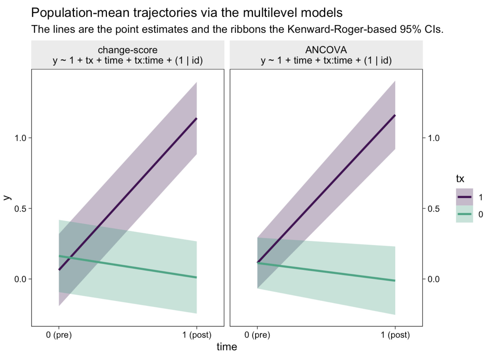
I can’t speak to what’s of clinical interest in your field. But if you can give me a way to make a plot akin to this (from the end of my blog post) with a conventional ANCOVA, I’d love to see it:
I want to make sure I understand the panels.
If those assumptions are right, then I need to see if I understand your goal:
The ANCOVA that conditions on pre and tx will give you E(post | pre, tx) as a continuous function of pre. That’s far more information and accounts for regression to the mean.
For the left panel, “multilevel ANOVA” would have been better wording than “change-score.” And yes, I agree the difference between groups at that baseline is noise, which was one of the subpoints in the original blog.
I believe we’re on the same page for the plot on the right. This is the one I currently prefer, and it’s the kind of plot I want. Frankly, I may have muddied the waters by even showing the left panel. It might have been clearer had I just copy/pasted the right panel.
My goal is to make a plot like the one of the right.
I suppose another way to get what I want, while honoring your points about the truncation, would be to fit a multivariate model along the lines of
where \nu, \tau, and a are the unconditional mean, standard deviation, and lower limit of the primary outcome at baseline. That way I’d still get my confidence intervals at baseline and could make my plot.
I was away yesterday and will be again today, so my apologies for the delays in further interactions here.
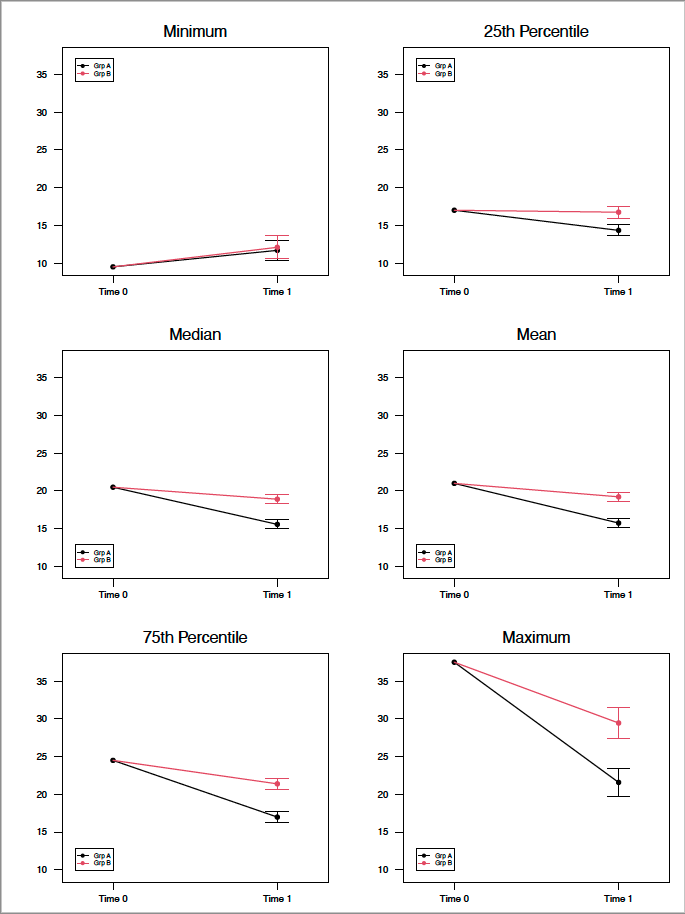
Since there seems to be something of a focus on the visual presentation, I wanted to share one of the ways in which I present these data, here in the setting of two time points as is being discussed. The same basic approach can obviously be applied to multiple post-baseline measurement designs.
To follow up on Frank’s earlier point, which is that the key question is, given a common baseline value for, in this case, two groups, where do they end up at the subsequent follow up time point, and what is the uncertainty in the estimate of the follow up measure?
Separately, using emmeans, I also generate the between group differences at the follow up, confidence intervals and p values.
Here, using simulated data, a single record per patient, and a simple OLS ANCOVA model of the form:
lm(Post ~ Pre * Group)
Generally speaking, we are primarily interested in the average treatment effect, thus use the mean baseline value to generate the estimates of the differential in the treatment effect at the subsequent time point.
However, I can also generate point estimates and confidence intervals for a vector of multiple baseline values, and present them in a single matrix of sub-plots.
In this case, I am using baseline values at standard distribution points, including the minimum, 25th percentile, median, mean, 75th percentile and maximum, for the sake of demonstration. Needless to say, these values can be replaced and/or augmented with other, what may be contextually or clinically interesting, baseline values.
The key takeaway here is that you can easily visualize the differing trajectories across the range of the baseline values, including hints at regression to the mean effects, and the differential in the treatment effects at follow up, given the interaction term in the model.
In either case, some food for thought.