(I edited all the quote marks to use proper backquotes for function and package names).
Your last question is the easier one. fit.mult.impute makes it so that any estimate or differences in estimates (contrasts) will automatically get the right standard errors accounting for multiple imputation. To my knowledge no one has taken this further to propagate imputation uncertainties to survival curve estimates. This is one reason I like full likelihood methods that make this much easier. If you don’t have too many distinct failure times you could the Bayesian ordinal regression capabilities of the rmsb package’s blrm function, which allows for left, right, and interval censoring. Then use posterior stacking with multiple imputation, which is more accurate than using Rubin’s rule in the frequentist domain. But the full semiparametric likelihood method doesn’t scale to more than a few hundred distinct failure times.
In terms of validation in the context of missing values see DOI: 10.1002/sim.8978 and these notes from others:
From Ewout Steyerberg
There have been proposals by Royston in the direction of stacking I
believe:
Recently in Stat Med more on doing analyses over all sets here
Daniele Giardiello d.giardiello@nki.nl 2017-03-28
I am Daniele a PhD student currently working with professor Ewout Steyerberg.
Here a list of the papers that can be useful for you:
Wahl (2016) - Assessment of predictive performance in incomplete data by combining internal validation and multiple imputation
Wood (2015) – The estimation and use of predictions for the assessment of model performance using large samples with multiply imputed data
In the simplest way, you could calculate the apparent c-index for each imputed data and average them to get the pooled apparent c-index.
In case of large samples the correction for optimism could be avoided.
Evidently, things are more complicated than I thought and I cannot use lrm or cph after fit.mult.impute as I thought. However, if I use lrm or cph on every imputed dataset and then validate (B = how many?) and average the resulting performance indexes and/or the performance optimism from each imputed dataset to a single value (e.g. Dxy or slope) – could that count as a reasonable internal validation of the whole model?
Most of my job can be handled with logistic regression but I also, in some situations, need Cox regression. In coxph you can do predict(cox.obj, type = ‘survival’) to get the individual survival probability. Is there a way to do the same thing with cph?
Large? Where the correction for optimism could be avoided.
The two projects with predictive ambitions look like this. Others mainly hypothesis testing or estimation.
n 3155 4989
Deaths 631 116
Deaths/15 42 8
Continuous var 2 2
Binary var (or 3 categories) 6 7
Large enough?
Again, thanks for your kind answer and I hope I got the backquotes correct this time.
If doing an external validation it’s just the coefficient of X predicting survival time in a Cox PH model, where X is the linear predictor developed from the training data. For internal validation the Cox model slope of the linear predictor is 1.0 and the bootstrap is used to estimate how biased is the 1.0, to derive a bias-corrected calibration slope.
Thank you for answering my question! I was also wondering how to plot calibration curves in R using k-fold validation. In addition to this, I was also wondering how c-index over time would be calculated using k-fold validation in R. Could you please advise on how these would be done?
I don’t have time-dependent c-index implemented (nor am I tempted to). For your first question the calibrate function has an option to use cross-validation instead of the bootstrap. Cross-validation typically takes more iterations than the bootstrap. Sometimes you need 100 repeats of 10-fold cross-validation to get adequate precision.
Thank you for answering this question! Could you please explain the difference between the calplot and calibrate function? I tried to create bootstrap calibration curves using both functions and both look different. I was wondering why this was the case.
When creating optimism corrected bootstrap calibration curves, the calibrate function with method='boot' as shown below would be used for 2-years follow-up:
Yes although that would be imprecise since you only fit 10 models.
Please read the RMS course notes for details about the calibration method, as well as reading the help file for calibrate.cph. Also note that I edited your post to use back ticks to set off code.
Notwithstanding the insensitive nature of the c-index, we have been challenged by a reviewer to generate bootstrap confidence intervals for a change in c-index between a “simple” and a “full” cph model where we are interested in added value. With rms::validate, one can get the optimism-adjusted (resampling-validated) c-index (i.e. (Dxy/2)+0.5) for both the simple and full models. For either model, one can bootstrap confidence intervals for Dxy (as shown in the following post: Confidence intervals for bootstrap-validated bias-corrected performance estimates - #10 by f2harrell). It is unclear to me (1) whether delta c would correspond to the difference between the two optimism-adjusted c-indexes (i.e. full - simple), and (2) how to bootstrap confidence intervals for this change.
There may be no reliable method to do this and interpretation thereof. Would greatly appreciate any help on these two points.
(For what it’s worth, we also reported output using the lrtest() function.)
Besides the issues already cited, the c-index has a nearly degenerate distribution because it is difficulty for it to fall below 0.5. Differences in c are likely to have odd distributions too. Normal approximations don’t work well for c.
I’m trying to conduct internal validation for my time-to-event model. When I use the calibrate function in rms, I get the predicted and observed probability of survival. How can I plot the predicted and observed probability of the event instead?
The plot method for calibrate doesn’t offer an option for cumulative incidence. But type rms:::plot.calibrate to see the code which will show you the points it is fetching from the results of calibrate() so that you can write the plotting code manually, taking one minus the y-coordinate.
Edit: I think I figured it out. More in my reply.
Thank you, Dr. Harrell. I’m not that familiar with R (I normally use SAS) so I’m wondering if you (or someone else) can tell where I went wrong with my edits to the function. Here are all the bits of code where I made changes (in bold):
[edit: incorrect code removed]
After making these changes, I’m getting “Error in calibplots2(cal_w1) : object ‘surv’ not found” (calibplots is the name of the above function and cal_w1 is the name of the object containing the calibrate function of my model).
In case anyone else runs into a similar problem, I got the function to give me the observed/predicted probability of event by making the following changes:
else {
    type <- "smooth"`
    pred <- 1-x[, "pred"]           #PB: add 1-
    cal <- 1-x[, "calibrated"]  #PB: add 1-
    cal.corrected <- 1-x[, "calibrated.corrected"]  #PB: add 1-
    se <- NULL
  }
I think I did this right but please let me know if I’m wrong!
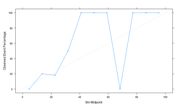
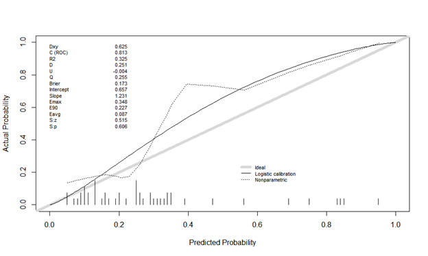
I need to ask about calibration again. I created the LR model and did a calibration plot on the test data (n=49). Below are two variants:
Here is the first calibration plot with binning using Caret. Looks like a true story!
The second is calibration plot using Rms, val.prob (predicted probability, class). The actual probability is odd, and it looks different. Is it plot without binning? Is there something I’m doing wrong?
Estimates from binning should be ignored. You can easily manipulate the shape of the calibration plot by changing the binning method, and it ignores risk heterogeneity within bins.
The minimum sample size needed to estimate a probability with a margin of error of \pm 0.1 is n=96 at a 0.95 confidence level. So it is impossible to do a model validation with n=49 even were all the predictions to be at a single risk value.
It is not appropriate to split data into training and test sets unless n > 20,000 because of the luck (or bad luck) of the split. What is your original total sample size and number of events? And how may candidate predictors were there?