Thank you very much for your quick reply. Can you embellish on this point? Let’s say you do not have any interactions in your model and are willing to assume the effect of the individual risk factor does not depend on the other predictors in your model, why is it more arbitrary (or less generalizable) to pick a cutoff for the individual markers based on your inference from the model (e.g. partial effect plot) than the risk score? Is there a good reference you would recommend I can read on this topic?
It is a mathematical necessity that the cutpoint on any one predictor must depend on the levels of all the other predictors. So it can’t be done. See Figure 18.1 in Chapter 18 of BBR.
Thank you.
Let’s say we had an interaction between a specific biomarker and treatment in our model and wanted to perform patient selection in a future trial which would consist of patients most likely to benefit from treatment (i.e. maximize the treatment effect). Is there a way to optimize this via a certain cutoff from your model? Here the focus is not on the risk score persay, rather on the subjects for which one treatment will outperform another, where intuitively I would have tried to base the cutoff on the value of the biomarker for which I see one treatment starts to perform much better than the other (I still don’t know how to identify such a cutoff). What would be your recommendation in this context?
If the outcome Y were to be continuous and you modeled it with a linear model, then the spline functions (main effects + interactions) used to fit the biomarker (so as to not assume linearity) directly estimates treatment benefit. When Y is binary then you have to choose between estimating relative treatment effects, e.g., relative odds, which makes things work just as with a linear model, or you need to estimate absolute risk reduction with treatment as a function of the biomarker level. This will be a function of the relative efficacy (spline interaction) and the baseline risk for control patients.
Dear all,
My question is about the ‘reliability’ of predictions for new cases of a penalized binary logistic regression model.
“The user of the model relies on predictions obtained by extrapolating to combinations of predictor values well outside the range of the dataset used to develop the model”
Given that the model was ‘trained’ using a high dimensional dataset, how should one inform the user about such predictions? Is there a recommended approach?
Thank you.
1 Like
That’s a really good question and one that has not been addressed sufficiently in the literature. There are three types of troublesome extrapolations I can think of:
- requesting predictions when a single covariate is outside the range of the training data
- requesting predictions when a pair of covariates is outside the bivariate range of the two in the training data
- requesting predictions for covariate combinations having collinearities that differed from the collinearities in the training data
The third problem is often more fatal than the first two. If X_1 and X_2 are positively correlated in the training data but for prediction you have a small X_1 and unusually large X_2, the predicted value can be quite wild.
We need a measure of how well the new covariate setting is represented in the training data, or how much of an extrapolation it represents. The only thing I’ve attempted works only when there are only 1-5 predictors: count the number of training observations having all 5 predictors within a certain tolerance of the new predictor values. We need something better than that.
1 Like
Thank you for your quick and insightful reply.
I have an additional question about the ‘rms’ package.
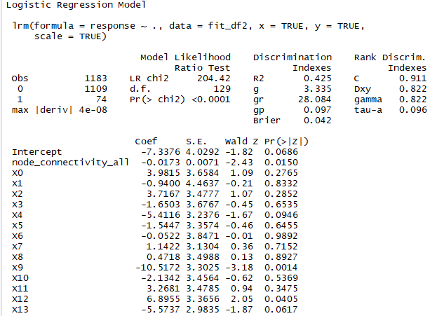
I am trying to fit a penalized binary logistic regression model with scale=TRUE.
As you can see, I have many predictors (>100) with 1109 negative cases and only 74 positive ones.
I attached a screenshot of a slice of the summary for this model.
mylogit ← lrm(response ~ .,x=TRUE,scale=TRUE,y=TRUE,data=fit_df2)
I made several attempts to find the best penalty for the model using pentrace, and more specifically by calling pentrace several times, each time with a different sequence. 236 gave the best results.
pentrace(mylogit, seq(200, 300, by = 1))
Best penalty:
penalty df
236 22.34846
penalty df aic bic aic.c
0 129.00000 -53.58375 -708.36309 -85.43560
200 24.69420 33.12450 -92.21855 32.02799
201 24.62183 33.12925 -91.84644 32.03910
202 24.54991 33.13366 -91.47700 32.04982
203 24.47846 33.13776 -91.11020 32.06015
204 24.40745 33.14153 -90.74601 32.07011
205 24.33689 33.14498 -90.38440 32.07970
206 24.26677 33.14813 -90.02535 32.08891
207 24.19709 33.15096 -89.66882 32.09777
208 24.12784 33.15350 -89.31479 32.10627
209 24.05902 33.15573 -88.96323 32.11441
210 23.99062 33.15768 -88.61412 32.12221
211 23.92264 33.15933 -88.26744 32.12966
212 23.85508 33.16069 -87.92315 32.13678
213 23.78793 33.16178 -87.58123 32.14356
214 23.72119 33.16258 -87.24166 32.15002
215 23.65486 33.16311 -86.90441 32.15615
216 23.58892 33.16337 -86.56946 32.16196
217 23.52337 33.16337 -86.23679 32.16745
218 23.45822 33.16310 -85.90637 32.17263
219 23.39346 33.16257 -85.57818 32.17751
220 23.32908 33.16178 -85.25219 32.18208
221 23.26509 33.16074 -84.92839 32.18636
222 23.20147 33.15946 -84.60676 32.19033
223 23.13822 33.15792 -84.28726 32.19402
224 23.07534 33.15615 -83.96989 32.19742
225 23.01283 33.15413 -83.65462 32.20054
226 22.95069 33.15188 -83.34142 32.20337
227 22.88890 33.14940 -83.03028 32.20594
228 22.82747 33.14669 -82.72118 32.20822
229 22.76639 33.14375 -82.41410 32.21025
230 22.70566 33.14059 -82.10902 32.21200
231 22.64528 33.13721 -81.80591 32.21350
232 22.58524 33.13361 -81.50477 32.21473
233 22.52554 33.12979 -81.20556 32.21571
234 22.46618 33.12577 -80.90828 32.21644
235 22.40716 33.12153 -80.61291 32.21693
236 22.34846 33.11709 -80.31941 32.21716
237 22.29009 33.11245 -80.02779 32.21716
238 22.23205 33.10761 -79.73802 32.21692
239 22.17433 33.10257 -79.45008 32.21644
240 22.11693 33.09733 -79.16396 32.21573
241 22.05984 33.09190 -78.87963 32.21480
242 22.00307 33.08629 -78.59709 32.21363
243 21.94661 33.08048 -78.31631 32.21224
244 21.89046 33.07449 -78.03728 32.21064
245 21.83461 33.06832 -77.75999 32.20881
246 21.77907 33.06197 -77.48441 32.20677
247 21.72382 33.05544 -77.21053 32.20452
248 21.66888 33.04873 -76.93834 32.20206
249 21.61422 33.04186 -76.66782 32.19940
250 21.55987 33.03481 -76.39895 32.19653
251 21.50580 33.02759 -76.13173 32.19346
252 21.45202 33.02021 -75.86613 32.19019
253 21.39852 33.01267 -75.60214 32.18672
254 21.34531 33.00496 -75.33974 32.18307
255 21.29238 32.99710 -75.07893 32.17922
256 21.23972 32.98907 -74.81969 32.17518
257 21.18734 32.98089 -74.56200 32.17096
258 21.13524 32.97256 -74.30586 32.16655
259 21.08340 32.96408 -74.05124 32.16197
260 21.03184 32.95545 -73.79813 32.15720
261 20.98054 32.94667 -73.54652 32.15226
262 20.92950 32.93775 -73.29640 32.14714
263 20.87873 32.92868 -73.04776 32.14185
264 20.82822 32.91947 -72.80058 32.13640
265 20.77796 32.91012 -72.55484 32.13077
266 20.72796 32.90064 -72.31054 32.12498
267 20.67822 32.89102 -72.06767 32.11902
268 20.62873 32.88126 -71.82621 32.11291
269 20.57948 32.87138 -71.58615 32.10663
270 20.53049 32.86136 -71.34747 32.10020
271 20.48174 32.85122 -71.11017 32.09362
272 20.43323 32.84094 -70.87424 32.08688
273 20.38497 32.83055 -70.63966 32.07998
274 20.33694 32.82002 -70.40642 32.07294
275 20.28916 32.80938 -70.17451 32.06576
276 20.24161 32.79862 -69.94392 32.05842
277 20.19429 32.78774 -69.71464 32.05094
278 20.14721 32.77674 -69.48665 32.04333
279 20.10036 32.76562 -69.25996 32.03557
280 20.05374 32.75439 -69.03453 32.02767
281 20.00734 32.74305 -68.81038 32.01964
282 19.96117 32.73160 -68.58748 32.01147
283 19.91522 32.72004 -68.36582 32.00317
284 19.86950 32.70837 -68.14540 31.99474
285 19.82399 32.69659 -67.92620 31.98617
286 19.77871 32.68471 -67.70822 31.97748
287 19.73364 32.67272 -67.49144 31.96867
288 19.68878 32.66064 -67.27586 31.95973
289 19.64414 32.64845 -67.06146 31.95066
290 19.59971 32.63616 -66.84824 31.94148
291 19.55550 32.62377 -66.63619 31.93217
292 19.51149 32.61129 -66.42529 31.92275
293 19.46769 32.59871 -66.21554 31.91321
294 19.42409 32.58604 -66.00693 31.90355
295 19.38070 32.57327 -65.79945 31.89378
296 19.33751 32.56041 -65.59309 31.88390
297 19.29452 32.54746 -65.38784 31.87391
298 19.25173 32.53442 -65.18370 31.86380
299 19.20914 32.52130 -64.98065 31.85359
300 19.16675 32.50808 -64.77869 31.84328
mylogit ← update(mylogit, penalty = 236)
However, after updating the penalty, LR chi2, d.f. and the p-value appeared to have extreme values.
For example, to the best of my knowledge, the d.f. for a penalized model should be lower than those of the original model. Running lrm with scale = False fixed this.
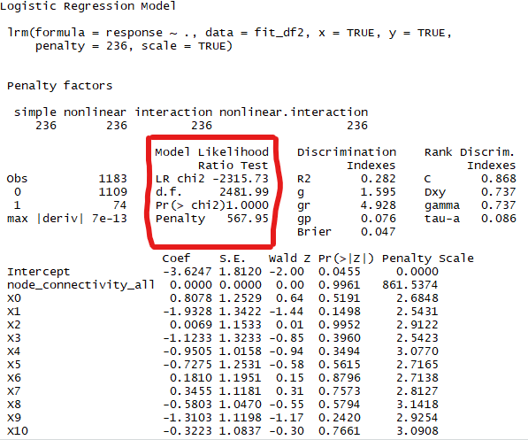
Is this really an error or did I simply not use the functions properly?
In your case the number of predictors exceeds the effective sample size, so many things go crazy. It has been shown that with small sample sizes you don’t have enough information to reliably choose the penalty. I would change to a data reduction (unsupervised learning) approach to reduce the dimensionality of the predictor space down to what the effective sample size (74 cases) will support. Consider among other things sparse principal components and aim for 74/15 = 5 variable cluster stores. Or fit first 5 PCs of whole set.
1 Like
I hope a non-technical, philosophical posting is acceptable here. I’m just now viewing the recorded lectures from the 2020 RMS short course. Thank you for making them available. I had planned to participate synchronously in May 2020 but, working for a county health department, I’ve been a bit busy this past year. Finally finding a few spare moments.
The Day 1 lectures included an interesting discussion about classification vs prediction vs action. This reminded me of “The Wolf’s Call,” a movie I coincidentally watched on Netflix just a couple days ago. It’s basically “Fail-Safe” but with the French Navy rather than the US Air Force. In the riveting opening scene, 4 French SEAL-type soldiers are in scuba gear swimming away from the Syrian coast toward a submarine that is supposed to retrieve them. The sub picks up a sonar signal, unidentified. The main character is the sonar operator, who has to “classify” the signal as a threat (enemy sub) or not. The very word “classification” is used repeatedly. The captain will take certain actions if it is an enemy sub (e.g. abort the mission, thereby abandoning the swimmers), and certain other actions if it is not (continue the mission and recover the swimmers.) So there is a “loss function”–a cost to deciding wrongly either way. The sonar guy eventually makes his decision, and the action ensues.
This seems to me like a good example of what Professor Harrell is talking about. The sonar operator announcees a classification–threat or not-threat. But his annoucemement is also a decision, because he knows what actions the captain will take if he classifies one way or the other. So the sonar guy’s “classification” includes an implicit and unexamined loss function. Might it have been better for him to announce his best professional estimate of the probability that the sonar signal is an enemy sub? Then the captain, who is supposed to be the real decision-maker, could use that info, along with his assessment of the loss functions, to make a command decision.
2 Likes
Great example!! Now I want to watch that movie if you recommend it. You are so right that the ultimate decision maker needed to be the one to translate the probability into action. And knowing the probability it is possible to make the decision a temporary one, if more information becomes available as the sub leaves the area and it’s not too late to return.
Oh, I highly recommend it, if you like tense political thriller action movies. I love nautical movies anyway; 11 years in the Air Force and I still like boats better than flying!
1 Like
Greetings. I am in the process of learning predictive modeling and am attempting to re-create the R code published along with the paper “Predictive performance of machine and statistical learning methods: Impact of data-generating processes on external validity in the “large N, small p” setting”. Specifically, I am running a bagged classification tree using the randomForest package. Following the R code in the appendix, I am getting an error code when I run the val.prob command, saying “lengths of p or logit and y do not agree”. Below is the code I am using. I would appreciate any insight into this error message and approaches to correct it. Thank you so much in advance.
bagg.1 ← randomForest(as.factor(OUT_MALIG) ~ REC_AGE_AT_TX + HF_ETIOL + CAN_WGT_KG + REC_MALE + CAN_HGT_CM + REC_CMV_IGM_POS + REC_CMV_IGG_POS + REC_HBV_ANTIBODY_POS + REC_EBV_STAT_POS + REC_DM + REC_RACE + REC_MALIG + REC_INDUC + REC_MAINT, mtry = 14, ntree = n.tree.bagg, importance = TRUE, data = data_train)
pred.valid.bagg ← predict(bagg.1, newdata=data_test, type=“prob”)
val.bagg ← val.prob(pred.valid.bagg, data_test$OUT_MALIG, pl=F)
in val.prob(pred.valid.bagg, data_test$OUT_MALIG, logit, pl = F) :
lengths of p or logit and y do not agree
The first thing to check is whether there are any missing values that were omitted thus shortening the vector of predicted values. Look at lengths of all vectors involved.
Thank you for the quick response (and please forgive my naivete as a non-statistician). I used the length(data_train) and length(data_test) commands to confirm they are both of the same length (n=33).
Show a high-resolution histogram of pred_valid_bagg. And is your test sample only 33 observations? That’s probably too low by more than a factor of 10. Are you using split-sample validation? If so that is very inefficient and requires much, much larger sample sizes.
So sorry for the confusion. The training set as 33,240 patients and 33 variables while the test set has 8,308 patients and 33 variables.
So there is something you’re not getting about the random forest predict function.
It looks like the ‘predict’ function is giving probabilities of each subject in the data_test dataset for either having (value=1) or not having (value=0) the outcome of interest (‘OUT_MALIG’) as follows (just an excerpt):
927 0.998 0.002
935 0.984 0.016
941 0.930 0.070
942 0.994 0.006
943 1.000 0.000
Then, I am running the ‘val.prob’ function (line of code below) with these probabilities from the random forest against the outcome in my test dataset. Is there an additional variable from the predict function that I am missing?
val.bagg ← val.prob(pred.valid.bagg, data_test$OUT_MALIG, pl=F)
I am not familiar with that predict function so you’ll need to do the work to make you retrieve a vector with one column and the number of subjects in the test sample as its length.
I was attempting to re-create code from your paper “Predictive performance of machine and
statistical learning methods: Impact of data-generating processes on external validity in the “large N, small p” setting” with my data to understand it better (specific lines from the bagged classification trees portion of the appendix code). I enrolled in your virtual regression modeling course in a couple weeks, so will learn more at that point. Thank you again for the replies.
pred.valid.bagg ← predict(bagg.1,newdata=effect2.df, type=“prob”)[,2]
val.bagg ← val.prob(pred.valid.bagg, effect2.df$Y,pl=F)