If there is only one non-absorbing state then the previous state is always the same (the non-absorbing one) and is redundant. See if that applies here.
I have a proportional odds model with four outcome levels: “0-4”, “5-9”, “10-14” and “>15”. The overall C statistic is 0.766 as given by the print() function for the model object. I obtain the same estimate of the C statistic if I use the validate() function and transform Summers’ Dxy to the C statistic. If I however use the val.prob() function for any of the individual levels of the outcome, I obtain a new estimate of the C-statistic for each level: 0.754 for “5-9”, 0.863 for “10-14” and 0.907 for “>15”.
Is there anything inappropriate about reporting outcome specific C-statistics if the proportional odds model will predominantly be used to predict one of the four levels in clinical practice? I would do this alongside the global C-statistic.
I am currently engaged in a research project with an ordinal regression model predicting an ordered response variable within the range of 1-9, I’ve been exploring various methods to estimate the variance of my model’s output (predicted probabilities associated with each class) During this exploration, I came across following methods:
- Bootstrapping
- Delta Method
- Bayesian methods like Markov Chain Monte Carlo (MCMC)
Given that Bayesian methods, such as MCMC, are commonly employed with small sample sizes and Bootstrapping requires generating multiple bootstrap samples, I believe the Delta Method would be a more suitable choice for my specific purpose. However after reading this paper : Using the Delta Method to Construct Confidence Intervals for Predicted Probabilities, Rates, and Discrete Changes, I wonder:
- What factors should guide my decision on the sample size for optimal results?
- What considerations should I take into account to avoid violating the assumption of asymptotic normality?
- Are there alternative methods for estimating the uncertainty associated with each predicted class?
P.S. Heartfelt gratitude to Dr. Harrell for providing us with this exceptional platform! @f2harrell
There is nothing wrong with getting c for different levels of Y other than a slight loss of precision. Note that val.prob is only for use on a sample that was not used in model development.
I don’t think the delta method has sufficient accuracy in many situations. And always remember that the delta method assumes that the confidence interval is symmetric. That does’t work well for probabilities outside of [0.3, 0.7]. Since Bayesian methods give exact intervals for any transformation of model parameters, it’s harder to get motivated to spend much time on frequentist approximations.
If you stick with a frequentist approach, I’d use the bootstrap instead of the delta method. The problem is which bootstrap from among the many choices. You’ll find differences in confidence interval accuracy among the various bootstraps.
Hi Professor @f2harrell,
I have a question about getting predicted means and confidence intervals when using the predict.lrm() function.
Note: fit is my fitted lrm() model and bfit is the bootstraped model obtained using bootcov() (e.g., bfit <- bootcov(fit, B = 500, coef.reps = T)).
Using ggplot(Predict()) seems straightforward:
ggplot(Predict(bfit, fun = 'mean'))
Building a nomogram is also working fine:
nomogram(fit, fun = Mean(fit), funlabel = 'Mean')
But I’m struggling with the code for getting the predicted means and confidence intervals on new data using the predict.lrm() function. I don’t know what the argument codes and the ‘design matrix X’ mean. Could you kindly give me an idea of what this code would look like?
Thank you.
I think that Predict or predict will give you approximate CIs. To get better CIs that use the bootstrap reps you may need to use contrast.
But if I use:
Predict(boot, fun = 'mean'),
then this will give me predictions on the mean scale and the CIs will be nonparametric percentile, right?
If I want predictions on the probability scale (e.g., Pr{Y>=j}, where j is the middle intercept), then I should use:
fun <- function(x) plogis(x-fit$coef[1] + fit$coef[middle intercept]),
and then:
Predict(boot, fun = 'fun').
Is that correct?
Thank you!
Predict (boot, fun = plogis, kint = j)
Hi @Elias_Eythorsson, thank you for your suggestion!
I run both,
fun <- function(x) plogis(x-fit$coef[1] + fit$coef[middle intercept]),
then
Predict(boot, fun = 'fun'),
and
Predict (boot, fun = plogis, kint = j)
I obtained the same point estimates for the predicted probabilities, but the lower and upper limits of the confidence intervals were different.
I guess the former (fun = 'fun') is using the standard estimated coefficients while the latter (fun = plogis) is using the bootstraped coefficients.
Does that make sense?
Thank you!
Also look at ExProb.
How?
Like this?
p <- Predict(boot, x, fun = 'ExProb')
But my model was fit using lrm(), not orm().
What about what I wrote in the post above? Is it correct?
Thank you
Calculating contrasts for a lrm() model:
m <- Mean(fit)
c <- contrast(fit, list(x = quantile(data$x, 0.75)),
list(x = quantile(data$x, 0.25)))
print(c, fun = m)
The relationship between X and Y is negative, in that going from the first to the third quartile of X results in a decrease in Y (as shown by the partial effect plot - test of association is significant: Chi-square of 13 with P < 0.001). However, that’s not what the contrast is showing, as the effect is positive. Also, going from first to third quartile or vice-versa results in different effect estimates with contrast(), instead of simply changing the signal of the effect (i.e., + and -). Also, there is no SE for the computed contrast (the output from print(c, fun = m) shows NA for the SE).
I wonder wheter this has something to do with the Mean() function?
I would appreciate any help on this.
Thanks
@f2harrell, please, could you kindly give me some guidance on the above?
Thank you
I hope others can. I have a heavy teaching load right now.
Hi @Elias_Eythorsson,
Do you have experience using the contrast() function for a lrm() model?
Any comments on the issue above?
Thank you
Dear all,
I’m using the TBI dataset (complete case analysis) from @Ewout_Steyerberg’s book, Clinical Prediction Models - 2nd edition, to fit an Ordinal (PO) Logistic Regression model, using rms::lrm(). My question is at the end of this post.
Outcome variable is Glasgow Outcome Scale (GOS, 1-5).
Below is the Hmisc::describe() output:
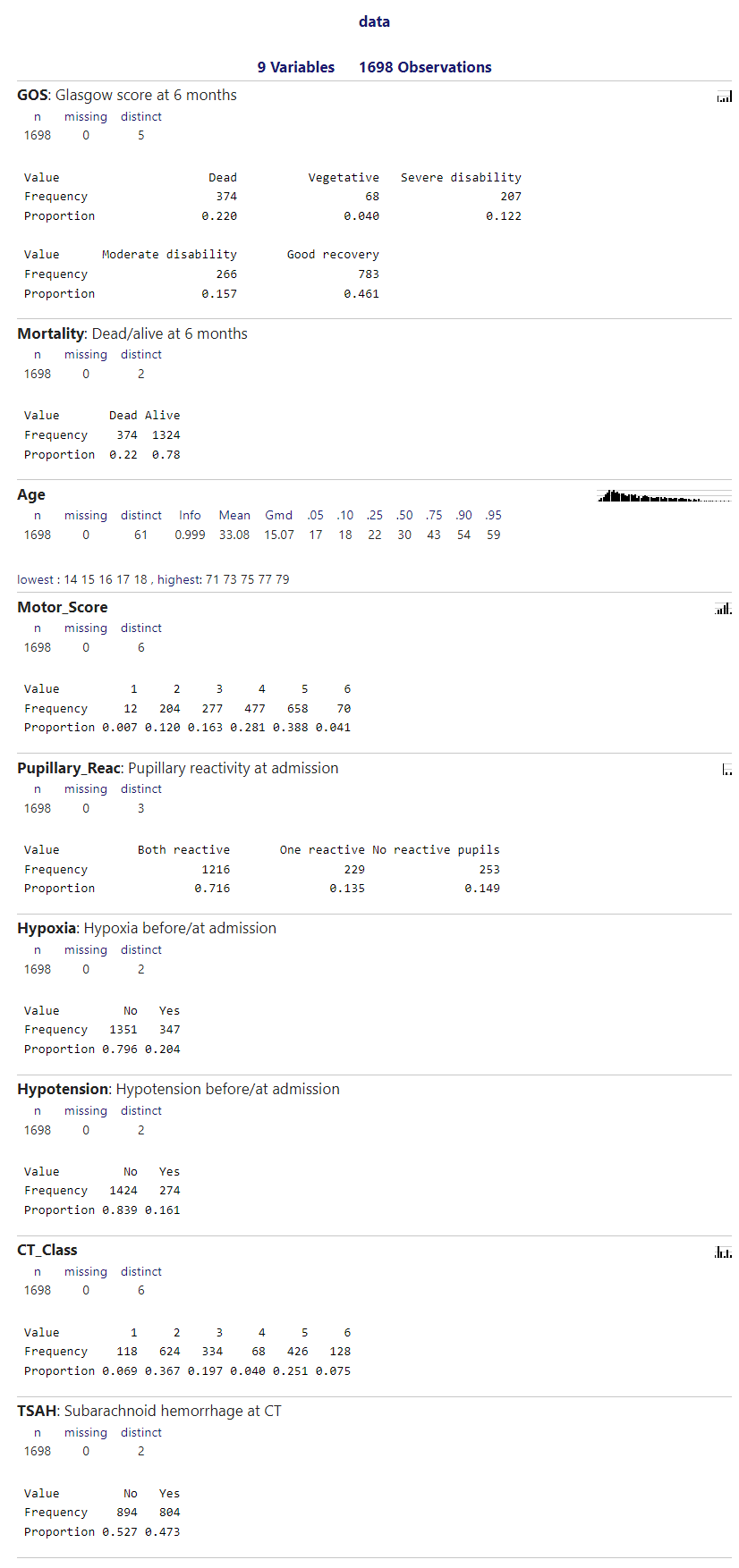
I have collapsed the categories from Motor_Score and CT_Class:
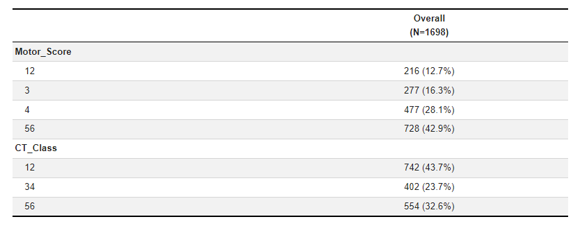
The model fitted for predicting GOS>=4 at 6 months was the following:
lrm(GOS ~ Age + Motor_Score + Pupillary_Reac + Hypoxia + Hypotension + CT_Class + TSAH, data = data, x = T, y = T)
Here’s the output from rms::validate():
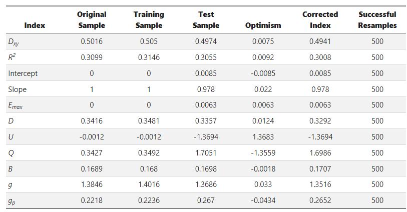
And from rms::calibrate():
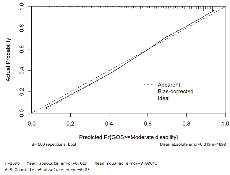
For comparison purposes, I’ve also fitted a Binary Logistic Regression model (GOS 1,2,3 vs GOS 4,5), which surprisingly (for me at least) seemed to outperform the Ordinal model:
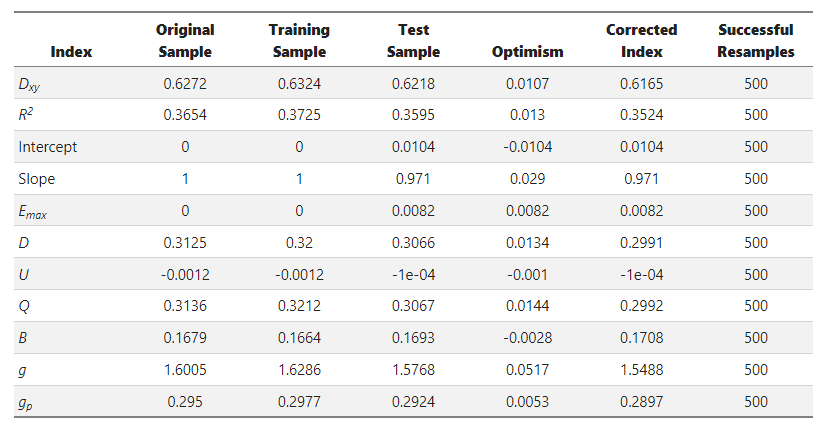
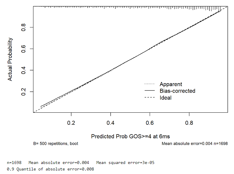
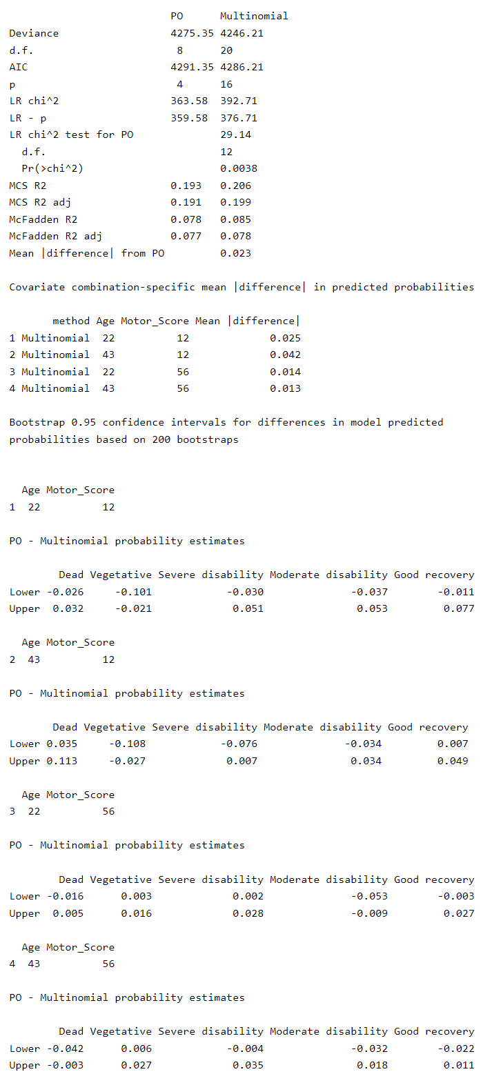
Could the reason for this be the fact that there’s evidence for non-PO in my Ordinal model?
Thank you!
There is evidence for non-PO but the degree of non-PO is only “semi-consequential”. The larger issue is that when you compare quantities such as c and D_{xy}, predicting an ordinal response is a much more difficult task than predicting a binary outcome.
Thank you for the reply Professor!
Would it be ok then for me to proceed with the ordinal model?
I ask not only because of the evidence for non-PO but also because of the mean absolute prediction error, which is 5 times smaller for the binary logistic model.
This is an extremely difficult decision. Both calibration curves are good. But AIC favors the multinomial model for prediction accuracy. I would slightly lean towards the multinomial model but not by much.
I was considering only the Ordinal and Binary models, and completely forgot about the Multinomial one (despite comparing it against the Ordinal). The calibration curves you see above are from the Ordinal and Binary models. From your last comment, it seems that you are not favouring the Binary model. Any particular reason? Many thanks!