It means that you have to calculate every possible combination of walking that path and sum everything up, to the best of my knowledge there is no built-in function for that. Am I right?
If so I might write one ![]()
It means that you have to calculate every possible combination of walking that path and sum everything up, to the best of my knowledge there is no built-in function for that. Am I right?
If so I might write one ![]()
Correct; it needs a little work.
I’ll try to rephrase:
My main interest is extracting the probability of having a primary event that precedes a competing-event (Need for a new function for that) or just having an event without experiencing a competing-event through the whole time-horizon ( Hmisc::soprobMarkovOrd() ).
Does the following notation seems right to you?
Pr ( (Y(t) = 1) ∪ ( (Y(t) = 2) ∩ ( (l<t)∪ Y(l) = 1 ) )
I think so. It’s worth deriving the estimand analytically but also to use a fitted model to simulate 100,000 covariate-specific outcomes and compute the proportion of the time that what you are interested in happened.
Another more of a technical question: Is there a way to calculate SOP for a state model that is considered to be an absorbing state for one state but not the other?
Let’s say I want to calculate SOP for a Primary Event, I cannot really code it as an absorbing or non-absorbing with soprobMarkovOrdm(), right?
Edit: If I understand correctly your code, defining an event as an absorbing ignores any prediction by the model and defines a vector of prob=1 for the absorbing state and prob=0 for all other states.
You cannot really do that for partially-absorbing state since a specific transition should be defined as 0 ( for our case P(1->0) ) but other transition-probabilities should be derived from the model.
That’s the relevant part:
Not sure I follow. An absorbing state causes the probabilities of being in that state to be set to 1.0 for the NEXT and all future assessment times. A partially absorbing state is treated as a regular state but will end up having very large effect of the previous state. Any state will be considered as absorbing or non-absorbing in all contexts.
I’ll try to demonstrate with some R code:
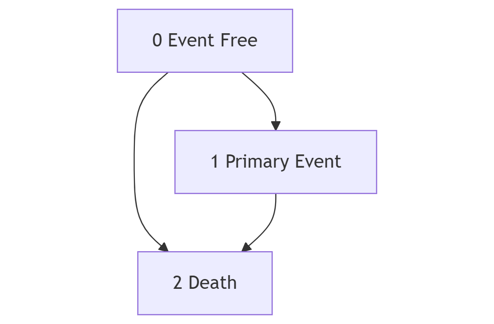
Let’s say once a patient experiences an event (1) he can be no longer in the state of “event-free” (0) but he might be in state “death” (2). I simulated data with no transitions from state 1 to state 2.
The transition probabilities from state 1 to state 0 are still greater than 0, the same is true for state-occupancy probabilities for different time-horizons even though it makes no sense:
library(VGAM)
library(Hmisc)
library(rms)
library(dplyr)
library(msm)

set.seed(123)

simulated_state_data <- data.frame(
  id = rep(1:10, each = 10),
  yprev =
    ordered(sample(
      c(
        "0 Event-Free",
        "1 Primary Event",
        "2 Death"),
      replace = TRUE, size = 100
    ))
) |>
  group_by(id) |>
  arrange(yprev) |>
  mutate(day = row_number()) |>
  ungroup() |>
  arrange(id, day) |>
  mutate(y = ordered(case_when(
    day == 10 ~ yprev,
    TRUE ~ lead(yprev)
  )),
  age = sample(1:100, replace = TRUE, size = 100)
  )


statetable.msm(
  y,
  id,
  data=simulated_state_data
)
#>     to
#> from 0 Event-Free 1 Primary Event 2 Death
#>    1           14               9       0
#>    2            0              22      10
#>    3            0               0      35


f <- vglm(
  ordered(y) ~ yprev + age,
  cumulative(reverse=TRUE, parallel=FALSE ~ lsp(day, 2)),
  data=simulated_state_data)

simulated_state_data[3,]
#> # A tibble: 1 × 5
#>      id yprev             day y                 age
#>   <int> <ord>           <int> <ord>           <int>
#> 1     1 1 Primary Event     3 1 Primary Event    85

# Transition Probability

predict(
  f,
  simulated_state_data[3,],
  type = "response")
#>   0 Event-Free 1 Primary Event   2 Death
#> 1 5.047615e-08       0.8050494 0.1949506

# State Occupancy

soprobMarkovOrdm(
  f,
  simulated_state_data[3,],
  times=c(1:7),
  ylevels=levels(simulated_state_data$y),
  absorb='2 Death',
  tvarname='day')

#>   0 Event-Free 1 Primary Event   2 Death
#> 1 5.047615e-08       0.8050494 0.1949506
#> 2 8.074696e-08       0.6481045 0.3518954
#> 3 9.687988e-08       0.5217562 0.4782437
#> 4 1.033224e-07       0.4200395 0.5799604
#> 5 1.033077e-07       0.3381526 0.6618473
#> 6 9.916276e-08       0.2722296 0.7277703
#> 7 9.254137e-08       0.2191583 0.7808416
Do I understand this correctly: There is a state s from which a person can transition to death but they cannot transition to any other state. So the state in question is not an absorbing state, but Pr(death | previously in s) is between 0 and 1 but Pr(state other than s and death | previously in s) = 0. This would require a model like the following. Let the death state be d and suppose there is one other state, c.
Pr(Y(t) = d | Y(t-1) = s, …) = expit(a + b[Y(t-1)=d] + …)
Pr(Y(t) = c | T(t-1) = s, …) = expit(a -1000[Y(t-1)=d] + …)
See if you can trick the covariate setup along these lines to do what you want. -1000 is just huge enough to make the probability negligibly larger than 0.
You understand correctly!
I’ll try to challenge your assumption with a simulation, but I have another question that pops into my mind:
Does variogram handle absorbing states well?
I made up an interactive and reproducible example with/out carrying forward death:
https://rpubs.com/uriahf/variogramabsorbing
While the shape looks good for this example, I wonder what will happen if we will extend heavily our time-horizon:
What will be the correlation between day 101 and day 1000 without excluding death cases? It will be close to 1 since an absorbing state on decision-point predicts perfectly the state in the following steps by definition.
It might be a weird correlation structure, with a lot of 1’s outside the more natural shape of a variogram.
A variogram should reflect the true correlation pattern even if there are absorbing states. But you’ll be hard pressed to find a non-multistate model that yields a correlation structure aligning with the correct variogram.
Some thoughts about chronic outcomes and OLM:
Sometimes we care about chronic outcomes that require some time to be classified as chronic.
It means you cannot model the outcome as time-to-event properly, because you should measure and wait for time to pass. You might give up the data in the follow-up and stick to ordinal results (Ordinal Regression) given baseline covariates solely, but I think it’s a waste of good data and meanwhile you would like to extract several decision points.
I think that OLM might provide a good solution while keeping risk extraction outside model development. That’s a huge mind-shift
For each day I can measure gfr levels and extract pr(Bad results after 3 months from index date). It’s more of a state-occupancy probability but not a direct outcome.
It’s a huge mind-shift for me, because clinicians want to know probabilities that are not well-suited for models but very convenient naratively.
It keeps the whole procedure quite agnostic. Any thoughts about that? @f2harrell
Hi all and @f2harrell,
I am a urologist (I also cover advanced genitourinary cancer), and clinical biostatistics is not my profession, so I apologize if this is a weird question.
I read your excellent article and have become a huge fan of the Bayesian ordinal transition model.
I would like to use the Bayesian ordinal transition model to re-analyze patient-reported outcomes (e.g., FACT-P, the Brief Pain Inventory, and Brief Fatigue Inventory) of patients who participated in RCT A and B for my future research plan. These RCTs evaluated the effect of new hormone drugs on advanced prostate cancer, so death could be the absorbing state. Should I include death as the absorbing state? Or just censor when death occurs? I think that although death is not part of PROs, it may be better to include it as the absorbing state.
Death needs to be an absorbing state, and that changes the estimands to explicitly be based only on observables. E.g. estimate P(PRO worse then y or dead | X); P(PRO better than y); P(PRO > y and alive).
When you treat death as censored you artificially increase the cumulative incidence, it’s the equivalent of saying the patient might get the primary event in heaven, but we don’t have any data about patients in heaven.
https://academic.oup.com/ije/article/51/2/615/6468864?login=false
Once you treat Death as an absorbing state, you should carefully state the probabilities of interest.
P(PRO worse then y or dead | X) , P(PRO better than y) and P(PRO > y and alive) are all path probabilities, and they are quite different from state-transition probabilities and state-occupancy probabilities.
@f2harrell correct me if I’m wrong, but no R function directly supports path-probabilities.
I’m not getting the difference between SOPs and path probabilities. Perhaps by path probs you are referring to the probability of ever being in a certain state. That can be derived from the totality of SOPs I think.
Thank you @f2harrell and @Uriah for your helpful responses! I will include death as an absorbing state rather than censoring it. In my research, I will focus on transitions between PRO states while alive.
That might work if you are interested in a Primary Event and do not care about the Competing Event happening afterward during the follow-up. This approach can be challenged concetually: I do not think that outcome in the form of 01111 is equivalent conceptually to 01222.
A patient suffering from CVD-event and experiencing some lifetime afterwards is very different than a patient suffering from CVD-event that dies right after. Weather the primary event is causally related or not, in terms of QALY the scenario is just different and in my mind should be at least explored.
How do you trick SOP for extracting an empirical estimate of experiencing a primary state that percedes an absorbing state during the follow-up?
The state occupancy probability stands for the union of all possible paths, Some API functions will be useful to extract specific paths while allowing the transition times to vary as long as they happen within the follow-up.
My best argument for OLM is that you separate the conceptual-production/medical/domain centered question from the statistical weird necessities:
If I care about change from baseline, I don’t have to encode change from baseline as an outcome. If I care about death within 5 days after cvd event, I don’t have to encode all other paths such as a patient experiencing CVD without death as “0”.
Interesting points. I wouldn’t say that SOPs stand for unions of paths.
Any quantity of interest can be estimated from the transition probabilties. A stepwise process will simulate 100,000 subjects’ paths then you can just count the number of subjects whose paths meet any criterion you can dream up. To do this analytically for all kinds of strange paths is more challenging.
Even if you want to solve it by simulation, you probably still need a nice interface!
How about something like:
Primary Event that precedes Death:
pathprobMarkovOrdm( model, path = c(0, 1, 2))
Primary Event with no death in the followup:
pathprobMarkovOrdm( model, path = c(0, 1))
Event Free in the followup:
pathprobMarkovOrdm( model, path = c(0, 0))
Wish we had that function already ![]()