Hi Andrew… I’m looking at data at the moment which has concentrations measured at 0,1,2,3 h + one or two more a few hours later. The rate of change depends a lot on when following the onset of the infarct the first measurement is made (the surrogate for that being onset of pain). Anything after ~12 hours beyond onset of symptoms can be in the excretion phase and change is harder to observe than the earlier release phase. I think that onset of symptoms should come into any model that is considering the prognositic value of change.
2 Likes
Agree John, I included time interval between sampling and onset in my initial attempts. There will be an abstract published in JACC from ACC in 2016 - I think I used a linear mixed effects model with a random term for subject, but could be mistaken. I will check it out but keen to look at this properly with some statistical experts 
http://www.onlinejacc.org/content/69/11_Supplement/246 Figure 2 shows distribution of troponin concentrations by classification and the estimates + CI are derived from a LME model as described above. I will have the code somewhere. My neck is firmly on the block now!
Interesting discussion. The majority of diagnoses of myocardial infarction are based on a clearly elevated single cardiac troponin concentration. Whilst serial testing will demonstrate a rise and fall, treatment will be initiated on the initial result. Serial testing is helpful in two settings though.
First, in patients with low troponin concentrations at presentation a second troponin concentration that is also low and unchanged helps to confidently rule out the diagnosis. Particularly important in patients with transient chest pain or presenting within 2 hours of chest pain onset. Here we define a plausibly significant change in troponin as >3 ng/L as this is outwith the 95% confidence interval of two repeated measures in a population without disease (based on Pete’s data). This change value is not used to diagnose myocardial infarction so analytical imprecision less important, but rather to identify those who should be admitted for peak testing (www.highsteacs.com).
Second, in patients with small increases in troponin concentration where the mecahnism is uncertain differentiating between acute and chronic myocardial injury with serial testing can be useful to guide subsequent diagnostic testing where echocardiography/CMR may be informative in those with chronic injury and coronary angiography helpful in those with acute injury. Here there is little agreement on what comprises a significant change (absolute or relative).
So when considering how best to model this we might need to consider that serial testing and change in troponin is being used for different reasons, and this is based on the initial measurement.
2 Likes
Really interesting data @chapdoc1 . I’m curious did you examine creatinine/renal function as a confounding factor ?
I feel as though there is a disjoint between the statisticians and the clinicians in the discussion above. I think, the reason why the clinicians are interested in change from baseline as well as peak troponin is because not everyone has the same baseline - for example people with renal dysfunction tend to have a higher baseline and perhaps altered kinetics due to the renal excretion of troponin. Bear in mind mild renal dysfunction can be relatively common, and some groups at risk for MI, i.e. diabetics, are also at risk of renal dysfunction.
It occurs to me that one way to deal with this could be to extend the model to include creatinine (or eGFR) as an explanatory variable.
That reasoning would dictate that the initial value be used in an analysis but it doesn’t follow that change from baseline should be relevant. It assumes too much (linearity, slope of baseline value on follow-up = 1.0). The best example I’ve every seen of this general phenomenon is with the most powerful prognostic factor in coronary artery disease: left ventricular ejection fraction at peak exercise. The resting LVEF is important, but change from rest to exercise has no correlation with long-term cardiovascular events. The LVEF at peak exercise has as much prognostic information as the entire coronary tree, and is summative. It automatically takes into account where the patient started at baseline. I realize the physiology is totally different for troponin, as is the timing of measurements, but this example serves as a warning to anyone who takes change as the proper summary of two variables. This is from this paper. And don’t forget this paper.
@f2harrell What do you think of including interaction terms for the baseline and current values for this kind of model?
, I suggest always started with a regression model that relates f(baseline) + f(current value) to the outcome, where f is a flexible transformation such as from a regression spline
Good on you Andrew for attempting to distinguish between type 1 and 2 early - it’s fascinating. When speaking with clinicians I usually ask some questions to try and help drive the model building exercise. These are the ones that came to mind:
- What factors do you use clinically to seperate Type 1 from Type 2 and are any of these available in the ED, therefore available to be put in a model?
- What clinical value is there in knowing early in the ED if a patient is Type 1, Type 2 or “merely” myocardial injury? (the “so what?” question).
- As a follow up to 2 (if the answer is “lots of value”) - how well would you need a model to distinguish between the 1, 2 or myo injury for it to be clinically useful?
So that is the reasoning used in practice and advised in clinical guidelines like uptodate article on the topic: UpToDate
So, the assumption is also not one of linearity, it is that the entire curve over time is shifted upwards. Reasoning being, the rate of elimination from troponin from blood is decreased. Thus the background level may be raised, peak level will probably be higher and the tail will probably be longer (governed by the pharmacokinetics/ pharmacodynamics at play).
From the comments there regarding troponin criteria in AMI, it seems as though this topic has been under-investigated, and I note from the second link you provided renal patients were specifically excluded:
It is apparent that none of the guidelines is truly data-based, and that they make very strong assumptions. And it it seems that no one has done a formal analysis of whether the latest troponin value may be interpreted independently of the earlier values. We still need a general analysis that utilizes the entire time course of troponins and estimates the optimal way to combine them, and how to weight the information over time. It may be that initial values do need some weight, but not as much as the most recent value.
99th percentiles of normals should play no role in decision making unless there are no prospective cohort studies with cases. Optimum decision making comes from risk-based analysis, not judgment against normals.
2 Likes
I wonder if this sort of analysis is helpful? It’s in a cohort of patients being assessed for possible MI & includes serial (0h & 2h) troponin. The diagnosis was a post-hoc adjudication based in part on on serial clinical troponin over a longer time period. It seems to me that the latest troponin adds the most to the model with a contribution from the first and interaction.
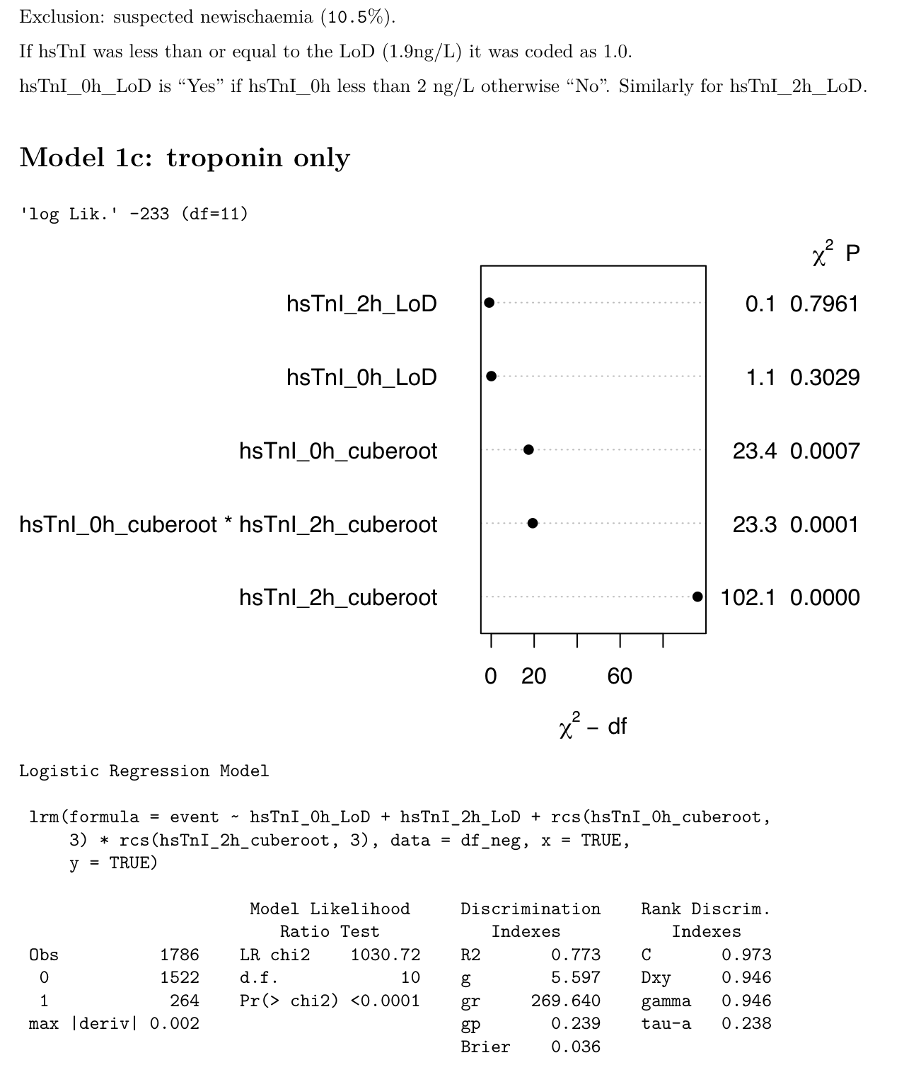
Very interesting, @kiwiskiNZ! I like the graph too, I take it as representing the weight of the individual variable in explaining the overall model? Would you share the code?
I wonder whether we get most of the information from the latest sample because time as a variable is somewhat built into the last sample - simply speaking, if it hasn’t gone up by time point 2h, you have all the information you needed in most cases to make a triage decision. I remember your IDI Plot demonstrating how little incremental value the hs-cTnI delta yields in classification when compared to the baseline sample. The regression model sort of tells you the same…
I really like seeing this analysis! The extremely high c-index makes me wonder if there was enough time separation between the 2h measurement and the final diagnosis, i.e., is there too much circularity? I have some suggestions for the analysis also.
- Instead of coding values below the lower limit of detection as 1.0, code them at the detection limit but add an indicator variable into the model for each of the measurements (looks like you already did that), indicating that it was below the lower limit. This allows for a possible discontinuity in the fitted relationship.
- See if the AIC improves by using 4 knots in the splines
- Use “chunk tests” to always combine the effects of continuous troponin with the effect of being below the lower detection limit, e.g.
anova(fit, x1, x2). - Plot the predicted values in a way to teaches us the role of the first measurement. One suggestion is to put the 2h troponin on the x-axis and make 5 curves corresponding to 5 values of the first measurement. Use the
perimeterfunction in thermspackage to blank out parts of these 5 curves where there are limited data, e.g., very low 0h and very high 2h. -
 Before fitting a model with indicator variables for lower limit of detection, fit models that have all needed terms under one entity by having more knots just after the lower limit. This is most easily done with a linear spline in the cube root of troponin, because it’s not restricted to a smooth first derivative so you’ll need fewer knots around the limit. To get knot locations, combine all 0h and 2h troponin values that are above the detection limit into a single variable. Compute 0.01 0.025 0.5 0.75 quantiles of cube root troponin and use those as knots. For the linear spline you can ignore the 0.025 quantile.
 -
For interaction terms, use the restricted interaction operator, e.g.
rcs(x1, k) + rcs(x2, k) + rcs(x1, k) %ia% rcs(x2,k)wherekis the vector of knot locations you computed above.
So far the results are supporting my findings in all other areas of cardiology: the final measurement needs to be emphasized and earlier measurements deemphasized. Don’t compute differences or ratios between the measurements, which gives equal weight to both measurements.
thanks Frank… I’ll certainly play. C-stats always high with trop (probably because of circularity if by that you mean because trop plays a part in the definition of MI).
I’d previous tried leaving the <LoD at the LoD (1.9) but made no difference (yes there is, as you suggested a while back, an indicator variable).
I’d tried 4 knots but it wouldn’t converge. Maybe I should play with the placement of the knots?
Compute knot locations using default quantiles, on the subset of patients that are above the lower detection limit. But I had a different idea about how to handle detection limits. Shortly editing what’s above.
library(rms)
plot(anova(fit))
I’ve code for ggplot too which I’ll dig out for you later.
1 Like
Forgot to say - a long time ago - I completed this analysis. https://www.sciencedirect.com/science/article/abs/pii/S0009898120300644
4 Likes
A blast from the past…thanks John!