Regression Modeling Strategies: Cox Proportional Hazards Model
This is the 20th of several connected topics organized around chapters in Regression Modeling Strategies. The purposes of these topics are to introduce key concepts in the chapter and to provide a place for questions, answers, and discussion around the chapter’s topics.
Additional links
RMS20
I am trying to create a Cox model for survival in oral cancers. Of the 10 covariates 4 don’t satisfy the proportional hazards assumption, with very low p-values.
As a result, the global p-value is also <0.05. Three of the 4 are the most predictive covariates. Some are categorical covariates (mainly present/absent) and one is a count (number of pathologically involved nodes).
I suppose I have to use stratification or time-dependent covariates. Are there any code examples in rms for these? I am relatively new to R. Happy to share the code used so far.
See this to start. And as is hinted at here different types of failure processes need different model structure. Try to reason from subject matter considerations. Is your example as simple as the acute vs. chronic disease patterns discussed in RMS? Do you expect the importance of risk factors to wane over time? If so then an accelerated failure time model that does not possess PH may succeed. Rather than customizing how different covariates fit by adding time-dependent covariates or stratifying (which works only for categorical covariates, in general), see if a different structure makes more of the predictors fit better.
For example if using a PH model results in 4 of 10 covariates not satisfying PH (especially if they are among the stronger predictors) by a log-normal accelerated failure time model fits well except for one covariate, the AFT model is preferred.
If I end up with a model with time-dependency in the way:
\lambda(t | X) = \lambda_{0} \exp(\beta_{1} X + \beta_{2} X \times \log(t+1))
Is it right, that I can plot this dependency just as a 3d plot and function of t and x?
So for example:
X has values from 10 to 40. (Follow-up) time is 10. And I get regression coefficients \beta_{1}=0.1 and \beta_{2}=4.
Then I can show my time and value dependency by plotting
f(x,t) = 0.1x + 4 x \times \log(t+1), \qquad 10\leq x \leq 40, \quad 0<t\leq10.
Just to look at how my dependency look like (for a rough view)?
And as a small addition, if the above is true:
If my x values are logarithmized before using in cox regression it would work just by transformation?
So the following to plot the logarithmized dependency:
f_{\log}(x,t) = 0.1x + 4 x\times \log(t+1), \qquad \log10\leq x \leq \log40, \quad 0<t\leq10.
and to show up the scale of the original non-logarithmized variable:
f_{\log}(x,t) = 0.1 \log(x) + 4 \log(x)\times \log(t+1), \qquad 10\leq x \leq 40, \quad 0<t\leq10.
Thank you. I will explore log-normal AFT models and get revert back in a few days.
Yes, assuming you used the special Cox PH partial likelihood function for time-dependent-covariates (i.e., you didn’t fit t as an ordinary covariate) you can interpret such plots.
For the other question, you have stated this as if you are “playing” with transformations rather than using a systematic approach that gives accurate inference because it penalizes for the number of parameters estimated. If you have enough events you can fit a tensor spline in X and t. See Gray for the use of penalized splines for this.
1 Like
Yeah, I had to dive really into this topic, but got the part using the special cox ph part.
The background just was that some time ago, I had the problem of very skewed distributed variable, so I logarithmized this variable. For this case a backtransform would have been needed to have it interpretable.
One additional question:
Is there any way to get the regression formula out of a restricted cubic spline in coxph?
Examplecode: coxph(Surv(time,event) ~ rcs(age,3) + sex, data=example)
How do I get the spline term to report it and to plot it like above mentioned? 
Use e.g.
require(rms)
f <- cph(Surv(...) ~ ...)
latex(f)
If using Quarto or RMarkdown you may need results='asis' in the chunk header.
With regard to transforming Y, semiparametric models such as Cox PH and proportional odds do not get affected by Y transforms that are monotonic (Cox unlike PO requires the transformation to be ascending for this to be true). If using a parametric model you can get estimates on the original scale using the smearing estimator.
1 Like
Thank you very much, I used coxph instead of cph and got error after error, but now its working 
Good to know, thank you for that hint!
Is there any workaround for the case with time-dependent covariates? Cause the tt addition just works in coxph, but latex seems to don’t work with coxph?
Sorry about that. I forgot to say that some time-dependent things work with cph, but not all.
1 Like
Although I have read plenty of hours in this forum, some questions regarding your course notes or to be clear some questions regarding “doability” came up my mind in the setting of coc proportional hazard modelling/coding:
- Is there a way to compute combined hazards?
So if I have a model with rcs how can I compute the combined Hazard of all rcs terms instead of the seperate ones (exp(coeff))? (not only by code also from the mathematical point of view)
- Is there a way to get “normalized” Hazards for all parameters in the model?
So instead of getting the Hazard for change in 1 unit of the variable, I would like to get the change of for example 1 quartile/tertile or something?
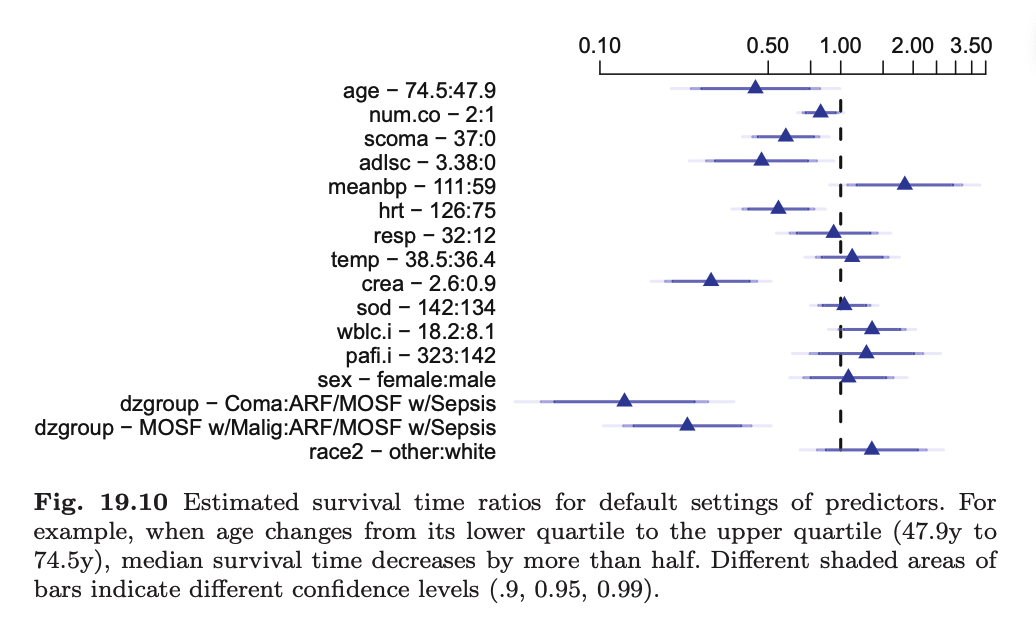
Beside a table I was also thinking of a plot like this one from chapter 10.9:
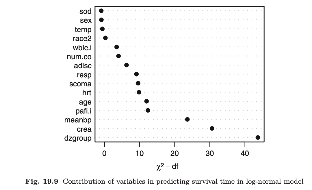
- There are these interesting variable contribution plots. Is there any way to get these too, for the case where rcs are in the model?
It is far, far better to either specify contrasts explicitly and get hazard ratio and compatibility intervals for them, or to use partial effect plots. Individual coefficients are just a means to an end. Inter-quartile-rank hazard ratios are decent defaults but only if the relationship is not very nonlinear.
1 Like
Well, I will follow your suggestion.
Do you have any suggestion/hint for the 1. one, so how do I compute the Hazard-ratio of for example age, if rcs(age,4) is in the model? 
Normally I would just compute exp(regr.coefficient) if I only have a linear term.
Does they add up in any way?
summary(fit, age=c(40, 60))
will compute the estimated HR for going from 40 to 60y, plus compatibility interval.
1 Like
thank you! Have to dive into the mathematical foundations of how it works behind, but for the first step this code will help! 
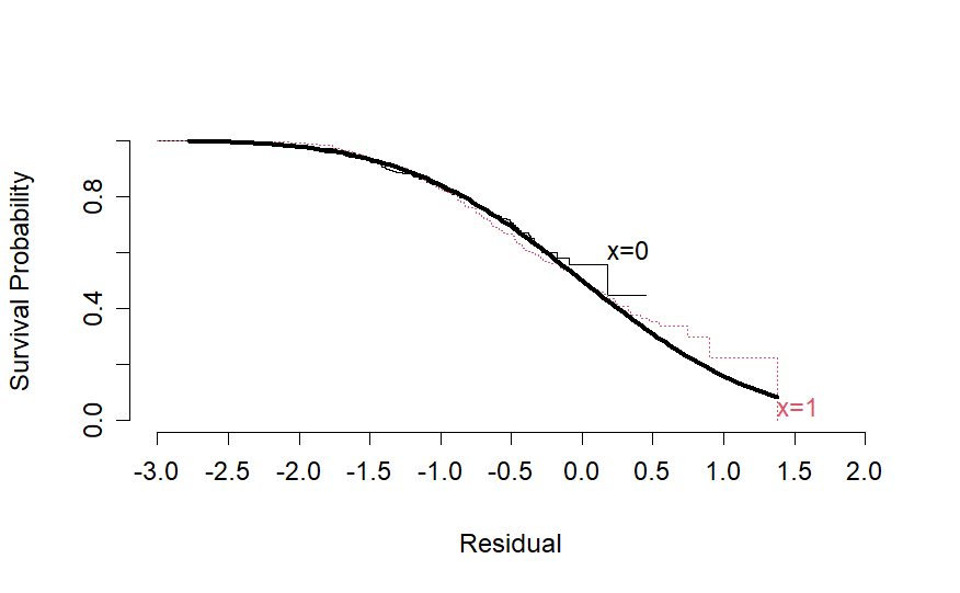
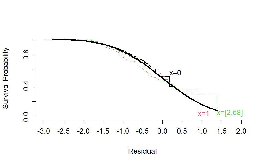
Dear @f2harrell, I tried your suggestion of using the log-normal AFT model as the proportional hazards assumptions were not satisfied for key variables in my model and by the looks of it this works. These are the residuals plots of the most problematic variables with cox ph that did not satisfy the proportional hazards assumption.
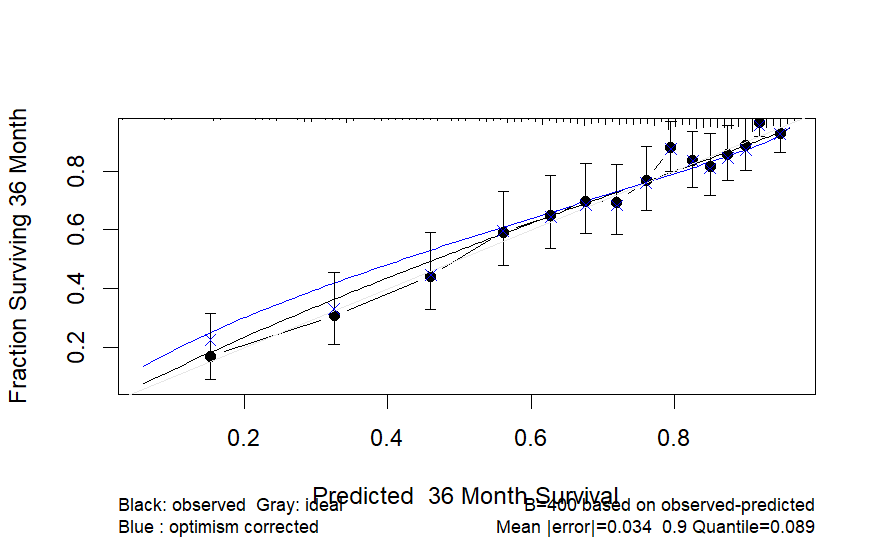
The final AFT model based on your code examples also gives equivalent LR and Dxy from the cox model with reasonably good calibration.
Thank you and will be grateful for any comments or inputs.
I’m glad the AFT model seems to fit adequately. On the calibration plot trust the blue curve and don’t trust stratified Kaplan-Meier estimates so much. The calibration is not quite adequate since those with very low predicted survival probability have better outcomes than predicted (overfitting; regression to the mean). But before we make that conclusion what is the predicted 36m probability such that there are 50 subjects with predicted values lower than that? That will inform whether to give much emphasis to the left part of the calibration curve.
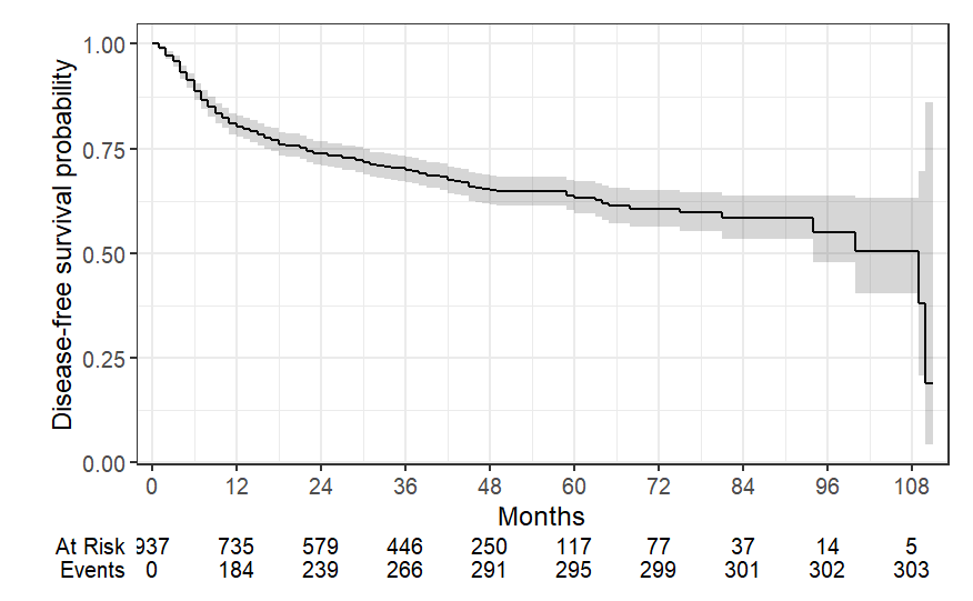
This is the survival curve @f2harrell
Does this answer your question?
No, I was asking for the 50th lowest predicted survival probability, so see which zone of the calibration curve (horizontally) is supported by data.