The 50th lowest survival probability is 0.23
So looking at where that falls on the calibration curve I’m worried about the accuracy of the model.
The optimism corrected values for Dxy = 0.48, R-squared = 0.19 and the model LR χ2 248.57, df = 22, Pr(>χ2)<0.0001 with 305 events in 937 individuals. Therefore it looks like a useful model with reasonably good discrimination. But the calibration at 36 months is off. How can miscalibration be fixed:
a) We have the correct sample size as per Riley et al. Will adding patients help?
b) Is it about choosing the right number of splines etc for each variable?
c) How likely is it that choosing a different time point for validation makes a difference?
and finally why did you ask specifically for the 50th lowest prediction probability?
A sample size of 50 gives you a reasonable basis for estimating the calibration in a given interval of predicted values. One could argue that 100 should be used.
What is the total number of candidate parameters (if any variable selection was done) and the total number of parameters in the final model?
No variable selection was done. This is a fully pre-specified model of 12 parameters. With rcs on some of the numeric parameters the df is 22.
So 22 parameters for 305 events. Using a rough 15:1 events:parameter rule of thumb that’s right at the limit. It’s worth going through this to get a better assessment. Riley has an R package for this and an online Shiny app.
We have considered the Riley paper while assessing the sample size.
The sample size was initially calculated for 20 predictors (with 12 actual predictors and some increase in df due to rcs). This was the output of the pmsampsize library.
NB: Assuming 0.05 acceptable difference in apparent & adjusted R-squared
NB: Assuming 0.05 margin of error in estimation of overall risk at time point = 3
NB: Events per Predictor Parameter (EPP) assumes overall event rate = 0.115
Samp_size Shrinkage Parameter CS_Rsq Max_Rsq Nag_Rsq
Criteria 1 897 0.900 20 0.18 0.759 0.237
Criteria 2 468 0.826 20 0.18 0.759 0.237
Criteria 3 * 897 0.900 20 0.18 0.759 0.237
Final SS 897 0.900 20 0.18 0.759 0.237
EPP
Criteria 1 15.47
Criteria 2 8.07
Criteria 3 * 15.47
Final SS 15.47
Minimum sample size required for new model development based on user inputs = 897,
corresponding to 2691 person-time** of follow-up, with 310 outcome events
assuming an overall event rate = 0.115 and therefore an EPP = 15.47
- 95% CI for overall risk = (0.264, 0.318), for true value of 0.292 and sample size n = 897
**where time is in the units mean follow-up time was specified in
However, while attempting the AFT lognormal model there were additional splines and the df increased to 22. For 22 predictor parameters the required sample size is 984 (so we are a bit short).
I have subsequently reduced the splines to keep the df to 20, with essentially no change in the shape of the calibration curve.
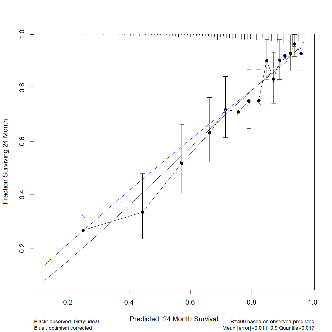
If I change the calibration time-point to 24 months, instead of 36, I get the following calibration curve, where the optimism corrected calibration is close to ideal. This time-point is also clinically relevant.
1 Like
It’s a difficult question becuase the residual plots look so good. Though this probably would not fit well I’d be interested in the calibration validation you get when a 14 parameter model.
Not sure whether this is the right place to ask or rather create a new topic. I fit a coxph model in an RCT, 2 groups, continuous time scale up to 180 days. I adjusted this model for baseline covariates to reduce outcome heterogeneity.
As I have to deal with ~25-30% missing data in the outcome variables only (as I only used baseline covariates for adjustment and there are no missing baseline data): Should I impute the outcome variables to get either more precision or power?
I know that it is not useful in mixed models to impute outcome variables when no covariates are missing and they are estimated with FIML-like procedures (see Enders, 2022). Unfortunately, there is little (at least as far as I know) literature on the same situation in Cox Regression. Yet, censoring should make this case somehow special.
Any thoughts?
Speaking in general imputation is not super helpful for outcomes unless you are (1) combining outcomes in some way or (2) you have a surrogate outcome that can substitute for a missing one, e.g., you don’t have the quality of life asssessment from the patient sometime but you have it from the patient’s partner.
1 Like
I had a question about Fig 20.4 on page 490 of RMS (2nd ed). How exactly is that plot being created? Two separate lines are plotted for sex, but the model it uses to generate the plot (f.noia) has no sex coefficient. When we print the model output, all we see are coefficients for age. I know the model stratifies on sex, but it’s not clear to me how the two separate lines are being generated. Can anyone shed some light on what’s happening under the hood? Thanks for any help!
A cool thing about the Cox PH model is that you can have an interaction between a modeled variable and an unmodeled (stratification) variable. I believe the fitted equation is given in the text. For an age x sex example you’d have two separate age effects, each having its own underlying survival curve so no apparent parameters for sex.
I’m new to prediction modelling and I think I have a reasonable understanding of the process for the binary outcome in terms of variable selection, assessment of calibration/discrimination, reporting of results in terms of nomograms, etc. However, I’m a bit lost for how to approach this for time-to-event outcomes using cox or parametric models, especially for the former where the baseline hazard is not actually estimated (how is risk calculated from this?).
Can anyone point me to some good resources - tutorials using R, papers, etc that illustrate the process of clinical prediction model development for the survival outcome?
Thank you.
With the Cox PH model the baseline hazard is estimated; it’s just that it is a two-phase procedure. First \beta is estimated, then these \hat{\beta} are used to make every person “alike” with regard to X so that then a Kaplan-Meier-like estimate of the underlying S(t) and hazard function \lambda(t) can be estimated. This complicates getting confidence intervals on S(t|X) but by this point everything looks like the result of a parametric survival model fit other than \hat{\lambda}(t) and \hat{S}(t) being step functions. The rms package tries to make the process look as similar for parametric and semiparametric models as possible.
I would like to ask some questions about model evaluation in a single model. In your book “RMS”, the validate.cph function is used for model evaluation.
My first question is, I understand that the c-statistic cannot be used to compare models. Do you recommend using your Harrell c-statistic to evaluate a single model? I did not see it in validate.cph, but many observational studies use it instead of logistic AUC.
Second, I noticed that you always use Dxy instead of c, although they can be calculated interchangeably. What is the reason for your preference for displaying Dxy over c?
Third, I have read in many methodology papers from BMJ and JAMA that recommend using the c-statistic to measure discrimination (I did not find other recommended methods in these papers). However, in validate.cph, I see many metrics such as slope shrinkage, the discrimination index D, U, Q. Can I understand that including these metrics in a table when I want to demonstrate discrimination and model evaluation would be better?
Fourth, I am reading the “RMS” book through your website, and I did not find a detailed explanation of the parameters in the validate.cph table. Perhaps I didn’t look in the right place. Can you tell me where I can find more information about the parameters, such as what slope shrinkage is, its range of values, and the meanings of Optimism and Corrected Index in the table?(My English listening skills are quite poor. Otherwise, I would really like to join your online course.)
Thank you for your assistance.
1 Like
I’m sorry I haven’t done a good job of documenting all the measures computed by validate in one place. The help file for validate.cph has the best available info.
I use D_{xy} because of its generality (and because in a linear model one can can use it alongside R^2) but you can switch back and forth with c.
c or D_{xy} is good for quantifying the pure predictive discrimination of a single model. So is a new adjusted pseudo R^2 printed by cph and documented here. In general we should prefer log-likelihood-based measures (especially once we get better at interpreting them) because of their sensitivity and generality.
Nono, your book and R packages are very excellent, but my statistical knowledge is limited, making it challenging to fully grasp many concepts. I’m doing my best to learn (recently delving into likelihood ratio materials; I have too many things I need to learn). I’ll go through the help files. Thank you very much.
1 Like
Professor Harrell, I would like to know if the rms package provides the calculation of Harrell’s c-statistic for survival models. I have checked the documentation, and I am unsure how to calculate it and whether the C statistic computed in Dxy is the same as Harrell’s c-statistic. If it is not, could you please guide me on how to calculate it? Thank you.
It’s standard output of the cph function in rms and you just need to linearly translate D_{xy} to get c.
Thank you very much, Professor Harrell.