RMS Semiparametric Ordinal Longitudinal Model

Regression Modeling Strategies: Semiparametric Ordinal Longitudinal Model

This is the 22nd of several connected topics organized around chapters in Regression Modeling Strategies. This topic is for a chapter that is not in the book but is in the course notes. The purposes of these topics are to introduce key concepts in the chapter and to provide a place for questions, answers, and discussion around the chapter’s topics.

Overview | Course Notes

A common cause of disappointment (e.g., uninformative nulls) is pursuing low-information (insensitive) outcomes. Thoughtful effort given to understanding and choosing high-resolution high-information Y will likely improve PTS.

A high-resolution high-information Y can flexibly accommodate the timing and severity of a variety of outcomes (terminal events, non-terminal events, and recurrent events); and the more levels of Y the better (fharrell.com/post/ordinal-info). The longitudinal ordinal model is a general and flexible way to capture severity and timing of outcomes.

The proportional odds longitudinal ordinal logistic model with covariate adjustment is recommended (the Markov model better still). With this ordinal model there is no assumption about Y distribution, and random effects (intercepts) handle intra-patient correlation.

The proportional odds ordinal logistic model can estimate the probability that Y=y or worse as a function of time and treatment. This modeling approach provides estimates of efficacy for individual patients by addressing the fundamental clinical question: ‘If I compared two patients who have the same baseline variables but were given different treatments, by how much better should I expect the outcome to be with treatment B instead of treatment A?

With this ordinal longitudinal model one can obtain a variety of estimates: such as time until a condition, and, expected time in state. The ordinal model does assume proportional odds but the partial proportional odds model relaxes this.

The model provides a correct basis for analysis of heterogeneity of treatment effect.

Bayesian partial proportional odds model, moreover, can compute more complex probabilities of special interest, such as the probability that the treatment affects mortality differently than it affects nonfatal outcomes.

Additional links

RMSol

Q&A From May 2021 Course

  1. Where do you think is the best place to start learning about Bayes, coming from a frequentist perspective? I know McElreath’s course is highly recommended, but I don’t think it ‘tells you’ the parallel approaches from the frequentist world - is there an (intro level) course or resource that does? dgl-I am working my way through the new Gelman book (Regression and Other Stories, Gelman, et al, (2021).), and am impressed with it. I recommend it. It has a balanced approach. fh-Kruschke does a lot of side-by-side Bayesian/frequentist analyses.
  2. Is there any limit to the number of states that the Bayesian Markov model can handle? Do you know if the models fitted using the Bayesian approach are comparable with the non-Bayesian Markov models fitted in the msm() package? Great questions. msm does not handle ordinal states, so every state is its own category and needs its own large sample size. With ordinal states there is no limit to the number of states as long as the proportional odds assumption is reasonably satisfied. You just need an good overall sample size.

Hi all,
A student and I would like to build an ordinal first-order Markov prediction model. Our data set has several hundred participants with outcomes measured at 6 time points across 4 months. The challenge we have encountered is that there are substantial missing values in the outcome variable (~15-20% at later time points). Consequently, there is a considerable proportion of missingness in the lagged outcome variable, which is a predictor in the model. The transcran help function has a great 6-step approach to imputing baseline variables using the time-varying outcomes. But we’re having trouble figuring out a way to multiply impute values for the time-varying lagged outcome variable. The Amelia II package allows for longitudinal imputation using a long data format. We can create a list of complete long-format data sets using the Amelia package, but we seem to lose the ability to capitalize on many of the desirable features of the rms package (fit.multiple.impute). Does anyone have suggestions for imputing missing values in time-varying predictors within the rms package?

This is a great topic. There are 6 approaches I can think of:

  • multiple imputation using tall and thin data, with standard multiple imputation algorithms
  • multiple imputation using wide data, e.g. Stata has a procedure for optimum within-person imputation looking forwards and backwards
  • full Bayesian modeling with missings treated as parameters (pretty complex here)
  • keep the data gaps and when measurements restart, sacrifice the first measurement so that it can be used as a lag for the 2nd measurement after the restart (not very efficient)
  • assume that last state carried forward is valid, i.e., that if a patient were measured instead of missing the measured value agrees pretty well with the last measured value
  • developed a complex recursive likelihood function for probability of the current state that is conditional only on the previous measured states

This is an active research area and we need to do a lot of work to select the best approach.

1 Like

Thank you, Frank! This is very helpful. I will follow the literature on this topic as this is an approach we plan to use often. At this point, we imputed using the mice package in the wide format, and rms seems to work seamlessly with mids objects. This Stack Overflow post was a helpful starting point. Our diagnostics for the MI model look good, but we will compare a few different approaches before proceeding with the primary analyses.

1 Like

May I leverage Ordinal-Longitudinal models for dynamic predictions?

My goal is to provide updated predictions, 1-7 days from index date.

While the soprobMarkovOrdm() provides very cool and informative predictions for each combination of time-horizon and state I would like to provide updated predictions for a given decision point.

It seems very natural to bayesian model, but I wonder if I can laverage first-order Markov PO model to do the same?

Since Markov models make it so easy to handle time-dependent covariates, I think there is a good chance that they are naturals for dynamic prediction. I’m thinking of dynamic prediction as a sliding landmark analysis, i.e., given that a person made it to time interval starting at t, what is their likely future outcome? Estimating the various outcome state occupancy probabilities just amounts to starting the Markov clock over, where the baseline state because the value of Y just before time t. Functions like the Hmisc package function that computes SOPs should work just fine.

Thanks! That’s what I had in mind.

I think that dynamic prediction might be beneficial in practice but I don’t see many of them in healthcare and I’m not sure why. For me it’s a great motivation to learn more of Bayesian statistics because it seems more natural to me to have a prediction that is being updated given a piece of new information.

Do you have any recommendations for Python packages that support Ordinal Longitudinal models?

I don’t keep up with Python. Hard to get motivated to re-invent the wheel when there are so many high quality R packages around. Note that as wonderful as Bayesian methods are, you can develop dynamic risk prediction models also with frequentist methods.

2 Likes

What other frequintist candidates do you find proper for dynamic predictions?
It took me a while to realize that I need dynamic prediction, but not necessarily dynamic model.

Another key point:
In your example you use discrete days (1, 2, etc…) but information tends to flow in non-discrete intervals, so my first thought was - are we losing information?

Decision-making enforces me to lose power not only in terms of translating state-order to binary decision (treat or not-treat) but also in terms of the possible gap between the updating-data-points and decision-making points.

Many dynamic prediction methods are available. Cascading overlapping landmark analyses are quite general. The other main approach is time-dependent covariates as in a Cox model. The information loss of binning into days will be important if the total follow-up is short or you really need to know which of two events occurred first on a given day.

1 Like

Thanks!
What about competing-risks model that handles time-dependent covariates? Isn’t it one step closer to multi-state model?

The time-dependent cox model handles well continuous time-events as can be seen here:

image

There’s also nice api in Python
https://lifelines.readthedocs.io/en/latest/Time%20varying%20survival%20regression.html

Side-note: I’m a huge R fan and I run a local R-users community in Israel, but whenever I want to push a model into production my collegues are always asking for Python API. Another drawback is that the documentation of the VGAM package is not promising, while I have the related book I still miss a github link that helps me to follow the code and a nice {pkgdown} / quarto documentation besides they ones that you made.

It will be also nice to have more package such as these under the tidymodels framework or just the tidyverse philosophy. There’s a nice implementation of cmprsk package here:

Would be cool to have something similar for OLM and it would be much easier to implement such models in production.

I avoid the tidyverse by all means to preserve my personal productivity :grinning:

Competing risk models provide hard-to-interpret risk estimates, e.g., the probability of having a heart attack that precedes death.

Another technical question, what do you do with variables once a patient is dead?
I saw in your example that all the variables are missing once the patient is dead (previous-state and age included).
Does OLM know how to deal with missing values? Is it true for all observing states?

I totaly get it!
I want to promote some of the ideas I learned from you, OLM included.
The {parsnip} package helps to promote some R code into production with an agnostic API:

I wish I could use that for OLM, maybe I’ll try to write my own wrappers in the future :slight_smile:

True, that’s why I tell my collegues they shouldn’t feel as imposters once they struggle with the concept - also some Causal jargon is implied which makes it even worse.

Multi-state perspective makes everything much easier to grasp from my point-of-view:

I’m working on extention for my package {rtichoke} that will allow to explore performance metrics interactively under different assumptions regarding competing-risks.

I think it’s much easier to think about competing-events in the context of decision-making in healthcare: You don’t want to treat a patient that is likely to die from another cause nor a patient that is likely to be event-free.

Once you regard these scenarios with utility jargon it’s much easier to understand. These assumptions are implied once you calculate the 1-KM/CIF/AJ estimate, they are all just another form of so-called “Real-Positives”.

https://www.ncbi.nlm.nih.gov/pmc/articles/PMC2611975/

1 Like

State transition models have the data terminate at the moment that one of the absorbing states is reached, so that is not a problem.

Regarding competing events models I still find them too conditional. I’d rather estimate Pr(sick or worse) than Pr(sick that precedes worse).

1 Like

I’m planning on piching for implementation of OLM in production :slight_smile:

Thought it might be useful to share key points from my POV:

  • OLM is natural for dynamic prediction (not to be confused with dynamic prediction model), important when facing several decision-points (same patient appears in different days).

  • Capable of dealing with different paths to Death (“competing event”) and deterioration, implies possible benefit for engagement such a consultion with an expert given a resource constraint.

  • Allows exploration for different components of state-occupancy in a given horizon-time by extracting transition probabilities.

Additional to the above I promise to provide some conventional prediction model outputs and compare performance. My metric of a choice will be average PPV for a given resource constraint each day.

One interesting key challenge would be to include some very different gaps for a given time-horizon in the followup. In hospitalization I can relate to every day seperately because blood-tests are quite common, but I want to incorporate longer time-horizons such as 5 years prediction.

Even for pure EDA it might be unusual experience.

PS: I opened an issue about soprobMarkovOrdm() function in {Hmisc} with some reproducible code, the function demands specific naming:

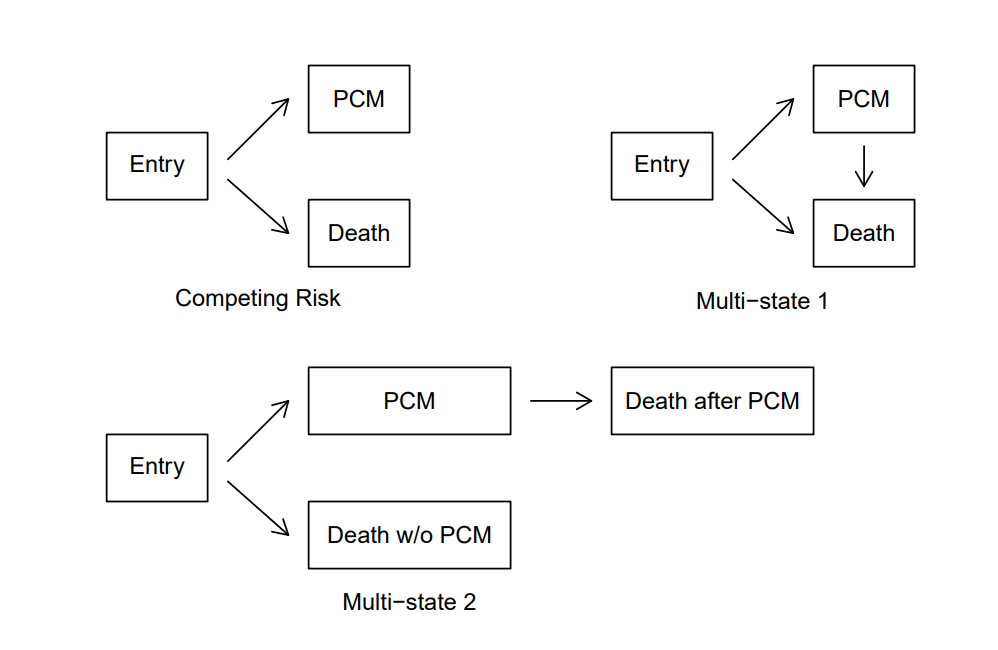
Question regarding competing risks under OLM framework:

What is the best approach, relate to death as a unified state or to add aditional state as “Death after Primary Event”?

My intuition goes with death as a unified state, but I’m interested in p(ever been in state Primary Event) and it’s not trivial to extract it. For the second option the estimation is nothing but the probability of state occupancy.

Another problem - how to order death-with-previous-primary-event and death-without-previous-primary-event?

Taken from this lovely article:

image

The states represent current status. Let the transitions take care of the rest. A person who transitions from well to sick to dead will penalize a treatment more than had she transitioned from well to dead, with death occurring on the same day in both cases.

How do you extract the probability of ever being in state “sick” until a specific time-horizon?

I know how to extract transition probability for next step and state-occupancy-probability for a step in the future, but not the probability for all kinds of specific paths such as healthy-sick-death.

I think this can be worked out using the same kind of recursive formula we use to compute SOPs. Let Y=0,1,2 = healthy, sick, dead. \Pr(Y = 0\rightarrow 1\rightarrow 2 | Y(0) = 0) = \Pr(Y=2 | Y=0 \rightarrow 1) \Pr(Y = 0 \rightarrow 1).