I think a better solution is to use biology and think hard about the “population” of SNP effects, then form a prior reflecting those. For example, instead of having a discontinuity at exactly the null, a horseshoe prior gives extreme favoritism to the null but does not downweight “big SNP effects” as much as lasso does. Biology and opinions about the “population” of SNPs over the genome may dictate a different prior than the horseshoe. The use of automatic priors (penalty functions) as with lasso and elastic net can be a problem.
Perhaps I am being unrealistic. I liked the BFDP because it is easy to apply against standard frequentist statistics and gives reasonably sensible results. I am as much interested in persuading colleagues to move on from P-value thresholds and given the failure of full Bayesian approaches to be widely accepted/implemented I was hoping that the simple approach might gain acceptance.
I see Bayes’ factors as getting in the way of understanding evidence more often than they help understanding. To me it is an unrealistic version of Bayes, since my world view is that there are few complete discontinuities in knowledge.
This is a helpful discussion for me, but not sure if it is to far outside the original topic. My view is that standard frequentist statistics has caused serious problems in biomedical science because the P-value and confidence interval are not answers to interesting questions. It is no use berating scientists and editors for continuing the status quo without suggesting a realistic alternative. Perhaps, the Bayesian alternative has not been adopted because the best is the enemy of the good. Do Bayes factors really lead to poorer statistical inference than what is currently used - apply the BDFP to most published nutritional/molecular/genetic epidemiology and one can rapidly understand why so few positive result replicate ? People find it very difficult to think about the priors (how does one come up with priors for subgroup analysis in clinical trials) and I think this is a major barrier to implementation.
Incidentally the prior distribution in the ANDROMEDA example of @DanLane911 seems rather unrealistic to me - it was based on a minimum clinically important difference which is rather difference to the likely true difference. If I run the @DanLane911 R-code but setting the MCID as the likely true difference with max of 0.9 then the plots look very different and a clinically important HR of (say) 0.8 looks rather unlikely 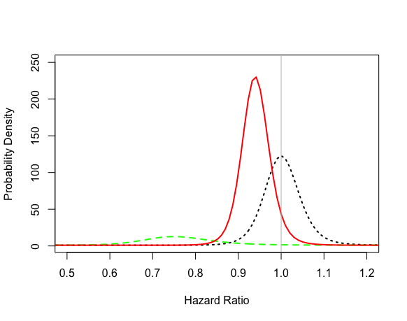
I don’t see the logic of bringing a “true difference” into the calculation. That’s what we’re trying to estimate. And regarding Bayes factors count me out. Try applying Bayes factors to statements about multiple endpoints or risk/benefit tradeoffs.
It sounds like we agree on the harms of P-values and confidence intervals. I would like to see more nuanced interpretations of results be a focus of biomedical science. But I agree with @f2harrell on the Bayes Factors - they are hard to understand and fundamentally don’t convey the information we/clinicians care about. Probabilities are the simplest and most intuitive estimates to be described, in my mind.
I’m not sure i understand what you are saying about the prior, or how you recoded it - the likelihood in my code was green but yours looks very different so not sure if you made an error in the coding or changed the colours (this distribution should be the same regardless of the prior)? Conceptually the way I coded it was so that the mean is centred on no difference (HR = 1) with a standard deviation that extends 5% past what the authors of this study hypothesized was a clinically meaningful difference. This prior encompasses a considerable range, but is rapidly overwhelmed by the data from the study itself so unless you add considerably more weight to your prior, it will not be modifying the likelihood much. You can modify this using @BenYAndrew’s app if you would like to test different hypothesis.
2 Likes
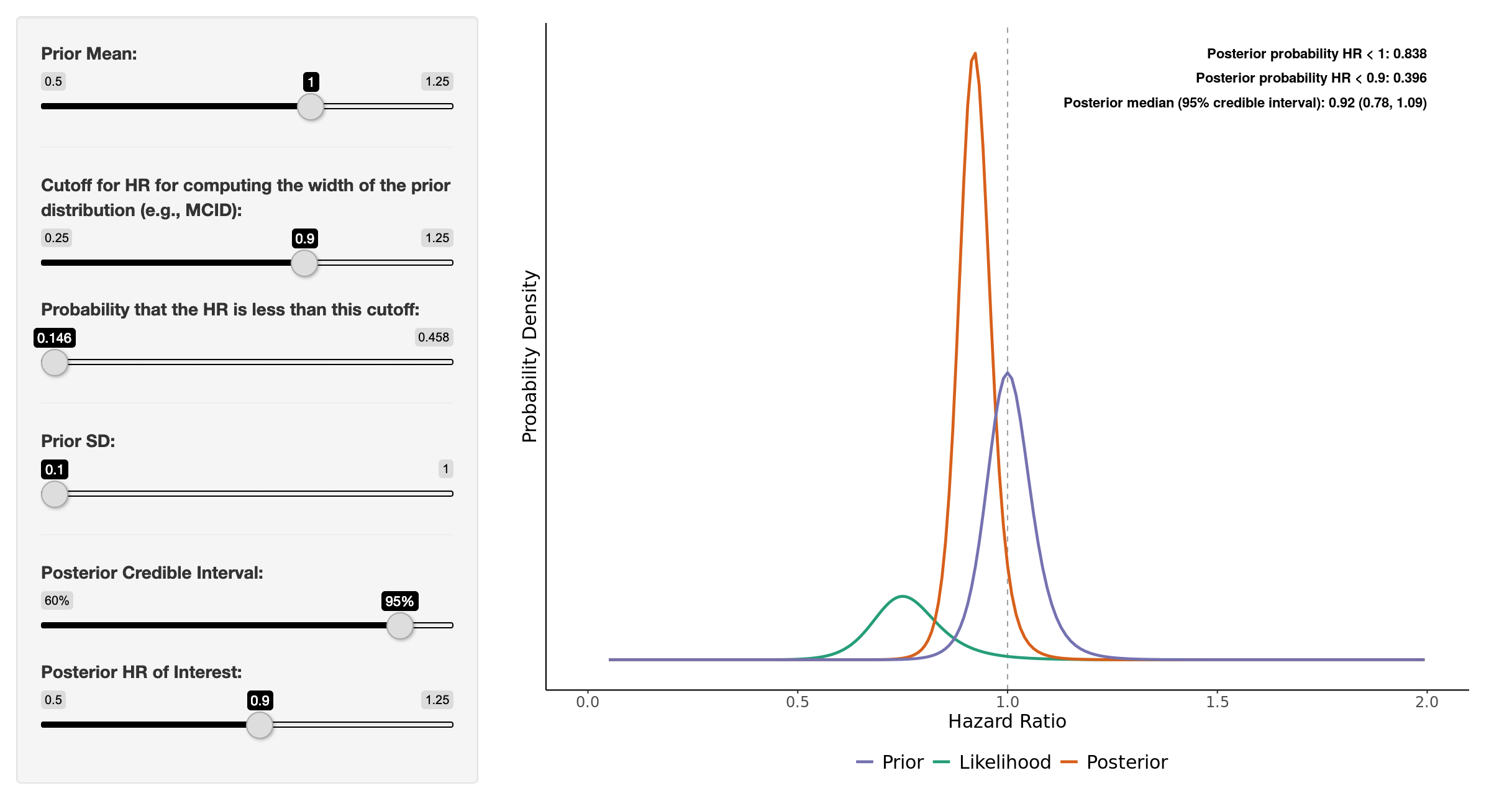
It looks like the prior @paulpharoah used was similar to the one in the attached image ( < 15% probability of the prior below HR 0.9) which, I think, represents a very skeptical prior. Even so, the posterior 95% credible interval is 0.78 - 1.09. You can now also visualize a heat map of Pr(posterior HR < user-defined HR) for a range of prior means/SDs using the app (image attached). Regardless, this type of interpretation of the study, in my mind, allows the clinician to make a more principled and informed decision when applying the evidence. It allows for more flexibility when taking into account different individualized “loss functions” that may alter how the evidence impacts decision making processes at different hospitals/clinics with varying resources, etc.

3 Likes
As I read the paper, a hopeless feeling began to invade me.
Consider these statements:
There was no evidence of violation of the proportional hazards assumption (Grambsch and Therneau test P = .07).
There was significantly less organ dysfunction at 72 hours af- ter randomization in the peripheral perfusion group (mean dif- ference in SOFA score, −1.00 [95% CI, −1.97 to −0.02]; P = .045)
By day 28, a total of 74 patients (34.9%) in the peripheral perfusion group and 92 (43.4%) in the lactate group had died (hazard ratio, 0.75 [95% CI, 0.55 to 1.02]; P = .06; …Among patients with septic shock, a resuscitation strategy targeting normalization of capillary refill time, compared with a strategy targeting serum lactate levels, did not reduce all-cause 28-day mortality.
Why do we bother measuring things to three places of decimals if in the end they are going to be interpreted like the height marker outside the fairground ride?
oTZ
2 Likes
Well put. This topic goes into more detail.
@DanLane911, could you explain how you came up with your skeptical prior?
Hi, everybody,
First of all, I have to introduce myself as the one who did most of ANDROMEDA’s statistical analysis, so take it easy on me. =)
before I jump in into the discussion of be or not to be Bayesian, I would like very much to hear about the following subject:
- In the Protocol, and later in Statistical Analysis Plan, we’ve planned the main analysis using Cox Model adjusted by some variables.
- As Ronan pointed
[quote=“RonanConroy, post:48, topic:1349”]
There was no evidence of violation of the proportional hazards assumption (Grambsch and Therneau test P = .07).
[/quote] we did not antecipate the lack of proportionality possibility, and did not addressed this in the SAP.
3. When we were writting the SAP, we discuss if we should change the main model approuch for a frailty model. And we decided that it will be better to keep main model as described in the Protocol and put frailty model as a sensitivity analysis.
So, first, the team was flawless, there were no loss to follow up, and the “almost” lack of hazard proportionality was there. Second, the icu’s heterogeneity was also present, and the frailty model was a better fit to the data. Should we have burned the SAP and adjusted a logistic regression? Or a log-binomial regression? Or a mixed logistic regression? In all cases, we would have achieved a significant result. What would you have done?
6 Likes
Nothing there makes me suggest that you drop the Cox PH model. A slight improvement would be to add random effects for sites but this is not absolutely necessary. Good work.
2 Likes
Yes - I centred it on a HR of 1 (0 effect) then selected a standard deviation which would extend the prior distribution 5% past the MCID selected by the study authors. In this case I had to calculate the MCID from the reported proportions then added the 5% to this measure.
Conceptually this is a skeptical prior as it makes no effect the most likely option, but then includes all values from 5% below the MCID to 5% above the opposite (MCID for harm).
3 Likes
In all cases, we would have achieved a significant result. What would you have done?
That kind of reinforces the point that the conclusions were inappropriate. It seems crazy to say “did not reduce all cause mortality” when other reasonable analysis methods would have found that it “did” (i.e. statsitical significance).
On another issue; why use a survival analysis rather than analysing the proportions survivng (logistic regression)? The aim of treatment is to increase the proportion who survive rather than to increase the time to death. Survivng a few more days is not really much of a benefit. This seems particularly problematic if (as I think was done here) deaths are only recorded up to day 28 (“The primary outcome was all-cause mortality at 28 days”). Also the sample size calculation reported in the paper is for analysing the outcome as a proportion.
Analysing the proportion of deaths at a specific time point does have the disadvantage that it is sensitive to the time point that is chosen. Generally people choose 28 or 30 days, on the grounds that most of the deaths will occur early and that’s what you’re trying to prevent, but there could be post ICU deaths thatwon’t be captured by the outcome. So results may differ depending on what time point is chosen. You can imagine you might get a significant result (the treatment works!) at 28 days but non-significant (it doesn’t work!) 14 days or 35. Survival analysis would be less sensitive to this but if the data are trucated at 28 days it still won’t take into account deaths that might occur later.
1 Like
Thanks for chiming in, and while I can’t speak for everyone here, I absolutely promise to go easy on you personally - this is purely an academic discussion about a really interesting trial with challenging results. I have worked on many projects where, for one reason or another, the final analytic choice did not leave me totally satisfied. I appreciate the complexities of all this.
Brutal. Absolutely brutal. No, I don’t think that you should have burned the SAP, and this illustrates one of the biggest challenges of RCT design & analysis IMO - we consider it very important to pre-specify as much as possible because of an overarching belief that any flexibility allows people to change things and pick whatever model gives the most convenient conclusion for them, but that comes at a cost of making it difficult to justify adapting when you have a statistically driven reason to believe a different model/tweak would be a better characterization of the data.
As often the case, I land very much in agreement with @simongates:
This is not to criticize you personally, @ldamiani, but rather the journal for rigidly requiring the use of phrases like “did not reduce mortality” to describe these results rather than a more reasonable “28-day mortality was lower in the capillary refill time arm (34%) than in the lactate arm (43%); HR=0.76, 9% CI 0.55-1.02, p=0.07” - which is factually true - without any use of the phrase “statistical significance.”
Simon brings up two other worthwhile issues:
I have wondered this at times myself - in trials of survival from a very acute condition, why not just use logistic for “30-day” survival or something, since loss to follow-up in that window is likely to be minimal and the true outcome at 30-days likely known for all participants - but is there any harm to using Cox instead of logistic?
I can’t speak to this for certain, but if deaths > 28 days are very unlikely to be affected by the acute treatment delivered in the trial, this doesn’t bother me too much. I know that some of the surgical outcomes reporting uses an outcome of “operative mortality” that is either “death within 30 days” OR “death within the same hospitalization” (so if someone has a series of post-op complications that keep them in the hospital for 40 days and then dies without having left the hospital, they still count as an “operative mortality”) - has anyone seen this used in ICU/critical care RCT’s?
3 Likes
If there is even one patient lost to follow-up before 30d I don’t see how to analyze the data without using time-to-event. You can use the event time (Cox) model to estimate P(surviving 30d).
5 Likes
To be clear, I don’t think anyone here is “blaming” you or your team. The blame for the inappropriate messaging almost certainly lies at the #TopJournals.
Congrats on this study. I for one am glad to see great this type of work arising from parts of the world which have historically not done so. Kudos.
1 Like
Dear Frank,
I don’t think this is the right way to put it. From the information given, the study was planned to detect a particular effect with some desired confidence. I must assume that the effect size, the power and the size of the test were chosen wisely and are clinically justified. Now, given these plannings, data was collected and and an A/B test was performed. This lead to the acceptance of the alternative “behave as if the mortality rates are the same for both methods”. The conclusion is not and can not be in question, as long as one accepts the chosen effect size, power and size. There choice might be disputable, and I suspect that the athorth have not provided a clear rationale for their choice, however. But in principle, the way they (technically) arrive at the conclusion to accept one of the alternatives is correct. The study was planned to deliver sufficient evidence under the assumption of the specified effect size (from 45% down to 30% mortality), with confidences defined by the given power and the given size of the test.
Your statement would be correct if the study had not been planned – if no effect size, power and test size were set, and some available data had been used to calculate a p-value, that would then have to be interpreted in the given context. Then observing p=0.06 might be indicating that the information from the data was not sufficient to interpret the sign of the log HR (the observed value is log 0.75 = -0.28, so the observed sign is a minus; however, the collected data may not suffice to take this serious – the sign cannot be interpreted with sufficient confidence, so to say).
The main problem, IMHO, lies not in the way the conclusions are presented. The main problem is that A/B tests (acceptance tests) are confused with tests of significance (rejection tests) and that the important meaning of adequate choices of effect sitzes, power and test sizes for A/B tests is unclear, unrecognized, or ignored – by authors, reviewers, editors and readers.
I agree with your last sentence completely. But I’m sorry to disagree vigorously with what’s earlier. Power is strictly a pre-study concept, useful in planning. Power can and should be ignored once the data are complete IMHO. And I question the choice of effect size in the original power calculation. It is not clinically meaningful. The effect sized used is above the clinically meaningful threshold.
To see that power should be ignored post study, consider the simpler case where Y is continuous so that the power calculation depends on the true unknown variance of Y. If the variance estimate used in the calculations turns out to be underestimated, the power calculation is just plain wrong.
I again claim this is a misinterpretation of the study’s main result and a misinterpretation of frequentist hypothesis testing, and is also ignoring the point estimate and compatibility interval. The compatibility interval (AKA confidence interval) includes a huge reduction in event rate and is not compatible with any more than a trivial increase in rate.
1 Like
Thanks for your response. It’s great that we disagree - that’s a point where I surely can learn something ![]()
I see that one can use power just to make sure to sample enough data that will likely be conclusive if the guess of the effect size (for which the power was set) was okayish. If I understood you correctly, then this is the “strictly pre-study concept”. However, I don’t think that this was in the mind of the inventor. If I am not misinterpreting Neymans work, the aim was to create an acceptance test, by specifying tolerable error-rates for two pre-specified alternatives. In the conventional setting, one of the hypothesis (A) is “the effect is zero” and the other (B) is “the effect is D”, where D is some finite, given, nonzero value that is deemd to be clinically relevant or of a size that would indicate to behave distinctively different than one would behave if there was no effect. These hypotheses are not stated to say that either the effect is exactly zero or that it is exactly D. These are only two scenarios under wich a certain behaviour would be adequate. Given a certain sample size, data allows us to decide to either “behave as if A was true” (accept A) or “behave as if B was true” (accept B), based on the losses associated with possibly wrong decisions. These possible losses are encoded in the power and the size (and in D).
The entire process of interpretation of (the possible results is put before the experiment. Afterwards, there is no freedom to interpret the data. The test statistic is either in the acceptance region of A or it is in the acceptance region of B. And these regions are, for sure, pre-determined by the power and the size of the test.
Agreed, but planning a clinical trial is not possible when the knowledge of nuisance parameters is missing or too vague. There simply is no point in doing an acceptance test in the first place when such things (including a reasonable D, or the losses associated with wrong decisions etc.) are not known. We obviousely never know everything precisely, but we should have some resonable guesses. If in doubt, one can (should) always choose the values in a way to minimize one of the risks (wrongly accept A or wrongly accept B - which ever is considered mor “critical”).
Again, the problems come in when the philosophies behined acceptance and rejection tests are mixed. We may ask if performing acceptance tests makes sense or is possible at all when it comes to research. My personal opinion is: no, it’s impossible!
The authors likely have actually done what you described. They used the power-calculation only pre-test to come up with a sample size that would likely allow the later interpretation of the data. Since the interpretation is put after the data collection, the power concept is irrelevant. If the authors then judge the “statistical significance” (p-value) of their data under the null hypothesis “HR==1” they must find that they can not reject this hypothesis, so the correct conclusion was that the data is not sufficiently conclusive to reject H0 (and thus to claim that the fact that their observed HR was lower than 1 is interpretable as a systematic effect of the method). So they actually did a rejection test, not an acceptance test. And yes, in this case I agree that power is irrelevant. But, to repreat me, not from the intended perspective of the Neymanian acceptance test. The rejection test does not know of the concept of “power” and “size”. It’s so confusing because there is no argument given why just p < 0.05 is used. If 0.05 is the planned size of the test, then I wonder why this is the criterion to base the conclusions (post-experiment!) upon and not, for instance, the planned power. I think it would be equally valid to conclude reject H0 because the “observed” power was lower than the planned power (or that the “observed” D was smaller than the planned D). It remains completely arbitrary unless a clear rationale is given why in this case, for this data, p < 0.05 would be ok to reject H0 but p > 0.05 (like 0.06 or 0.1 or whatever) would not.
Interpreting point- or interval-estimates is possible only in a Bayesian way of thinking (here implying a flat prior). I agree that, in research, we actually always face estimation problems and simply circumvent a proper analysis by falling back into meaningless or mindless frequentist testing routines. It would be far better to conclude studies with a statement about how much we learned from the data of a study regarding some effect (or model parameter) than to end with a dichotomous pseudo-decision between “significant” and “non-significant”.
Do you still think we disagree?