@DanLane911 and I have been working on a broader application of the Bayesian re-analysis application that was originally built for the ANDROMEDA-SHOCK trial. I was hoping to get some feedback on usability and ideas for improvement given that this is the audience most likely to use this type of tool. Right now the app is very much still under construction, but most of the basic functionality is implemented.
If the above link is not working, you can run the most recent version on your local machine (assuming you have Shiny installed) using: runGitHub(repo = “bayesian_trials”, username = “andrew10043”)
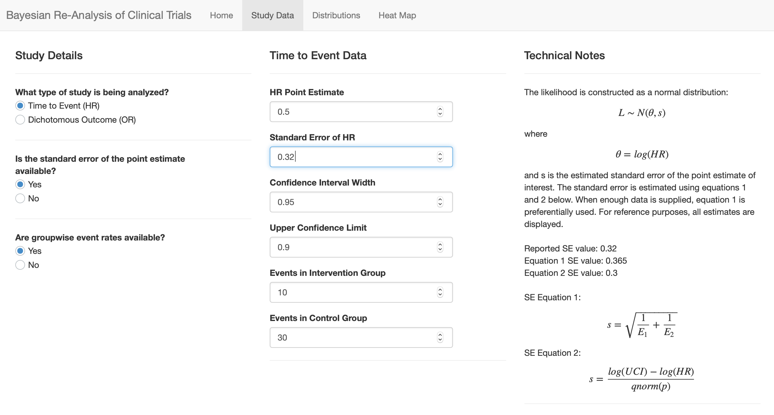
So glad you continue to generalize this! It’s neat that you are asking for the number of events separately by treatment group, which I assume you are using to get a more accurate estimate of the standard error of the log hazard ratio by summing the two reciprocals of number of events. It would be good to include in the output the comparison of the standard error using this approach with that obtained by backsolving from the confidence interval for the log HR.
One cosmetic suggestion that is a very minor thing is to see if shading tail areas or equivalence zones in the posterior densities would add something.
I had actually included event rates to allows for interpretation of studies with dichotomous outcomes (there is a drop down box that allows you to select HR or OR which then toggles the entry fields). In the current version, the standard deviation of the log HR likelihood is estimated as:
s = \frac{log(UCI) - log(HR)}{qnorm(0.975)}
I see, though, that the standard error of log HR can (as you point out) be estimated using:
It’s as close as we have to a gold standard, so I would use it but list beside it the back-computed s from your first formula to show the reader a check. Maybe better would be to use log(UCL) - log(LCL) and to adjust the denominator accordingly. This would be very slightly less affected by roundoff perhaps.
If the user finds that the SE of the log HR was published, they should be able to enter that and to have it compared with the other 2 SE estimates.
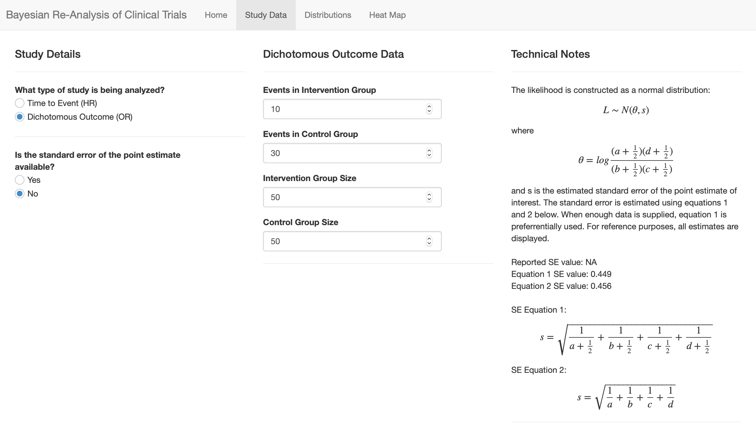
That’s right, for the log OR. I don’t routinely use the 1/2 but I think that using it is better than not using it. You might ask for the published SE and recalculate it for the user with and without the 1/2, then say you’re going to use the 1/2 for what follows. Of course what we really want is adjusted OR and HR but then we don’t have simple formulas. Anyway, RCTs shy away from these better adjusted estimates, preferring to lose power instead of having to get a statistician to explain the result .
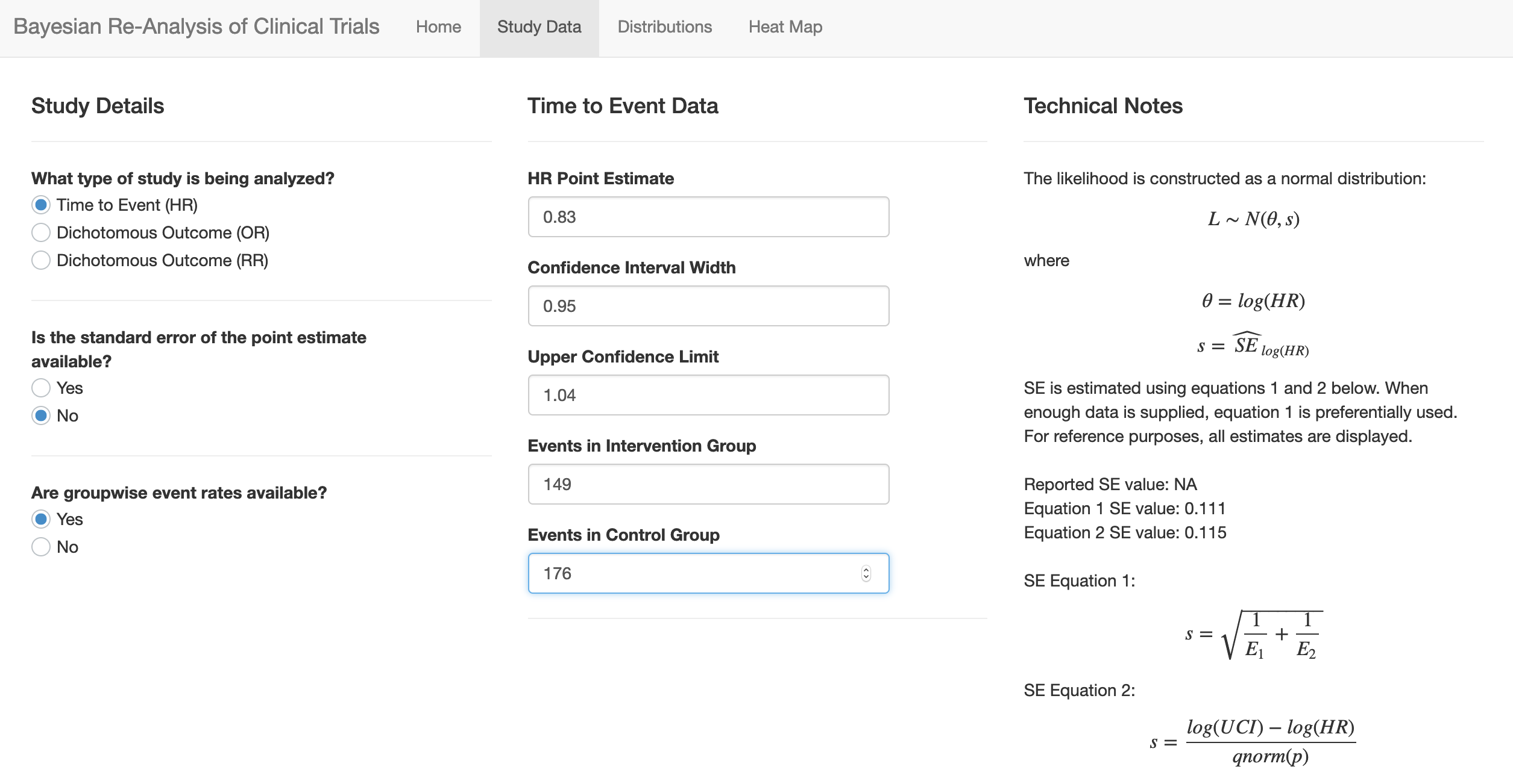
A few of these updates have been implemented (screenshots attached). There is now a separate “study data” page that uses user input to dynamically guide data entry. As @f2harrell recommended, the various approaches to estimating the SE of the point estimate have been included, and the best option is chosen to build the likelihood. The other values are displayed for the user’s reference. Still working on some of the aesthetic changes as these are less in my wheelhouse.
They use a HR, not RR or OR, so not sure which to choose.
Also, and this is possibly a moot point, but I guess might affect my interpretation.
The study showed that lowering BP reduced mild cognitive impairment (
I think, from my prior knowledge, MCI is strongly linked to dementia, and is on the causal pathway.
Am i allowed to use that information to adjust my prior? Knowing the study reduced a variable on the causal pathway to the primary outcome?
I’m neither a clinician nor a statistician, but hopefully I can help!
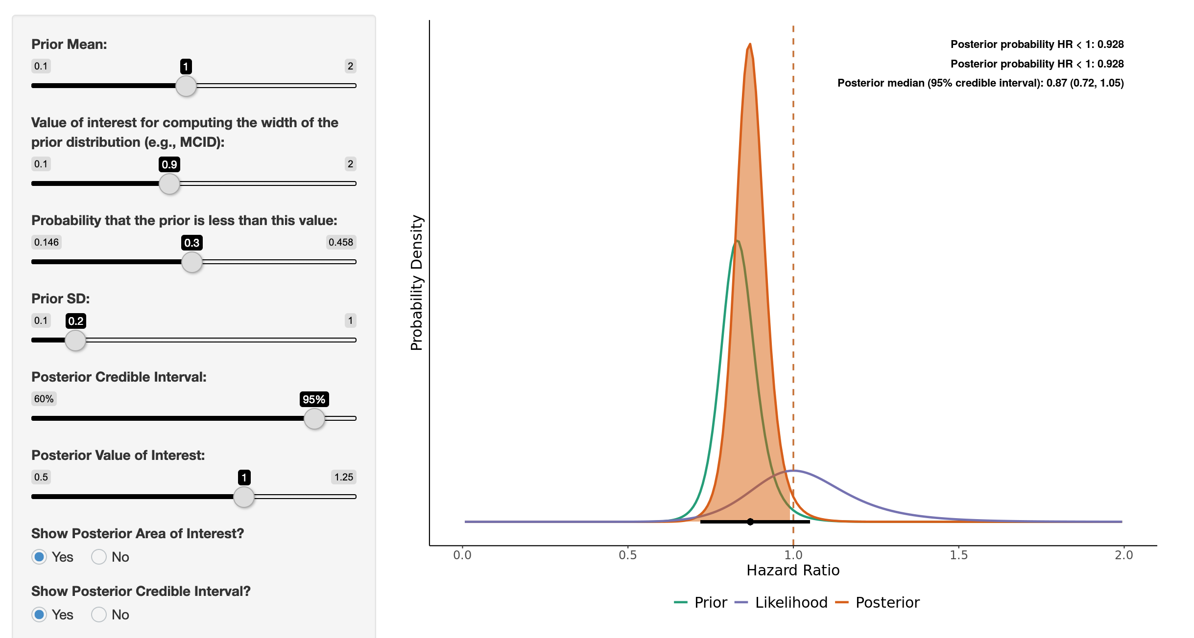
Using the “probable dementia” outcome, I would set up the app as shown in the attached images (you can play with the prior here). You can use the HR + event rates to get a good estimate of the standard error for the log(HR) which helps to reconstruct the likelihood function.
I would agree that causally MCI is on the path to dementia (although some etiologies of dementia may occur independently of MCI, I suppose, such as a more abrupt onset vascular dementia for example). I think when setting priors for this study it would be incorrect to use information gained from the study itself (e.g., using the MCI outcome to change prior for the dementia outcome analysis). Moving forward it would be reasonable to use the signal for MCI when constructing a prior for dementia studies, I would think, given that we theorize that MCI is an intermediate step on the causal path towards dementia.
I’ll let the more experienced group chime in, though, as I suspect there is more to add!
Just a really great example of this sort of work. My fiance is an old-age psychiatrist, so hence my (vague) interest in dementia as an ID clinician.
I showed her last night the influence of her skeptical prior on the results and it really became clear how to combine her prior information with this new work.
As you say about the MCI adjusting your dementia prior - I agree - I guess you can’t use it!
I am a surgeon and PI of a recently completed RCT. We randomized 308 patients to two treatments for a condition with a high mortality. We planned to test for an interaction between treatment and the preoperative diagnosis of two conditions (A and B). There was a significant interaction (p=.03). In condition A (n=95), the adj RR for benefit with treatment L was 0.81 (0.64-1.04); adj risk diff was -16% (-35,3). In condition B (n=213), the adj RR for benefit with treatment L was 1.1 (0.95-1.3); adj RD 7% (-4, 18). Our target journal is/was NEJM and after reviewing many recent papers, I’m afraid we might have to conclude no statistically significant difference in outcomes, but perhaps treatment L appears to be clinically significantly favorable for subgroup A.
Using neutral prior, our Bayesian posterior prob of benefit with treatment L for subpopulation A = 97% and for subpopulation B = 20% (i.e. 80% prob of benefit with the other treatment).
I’m struggling with how to present these findings in a manuscript that would properly account for both statistical methods. We did prespecify both methods, with frequentist approach being primary.
Any advice to this surgeon who wants to get the message “right” and has limited experience with these issues. Also, JAMA seems more Bayesian-friendly, but I have to admit that I like the NEJM impact factor. NEJM has also published the only prior trials in this disease area.
Welcome to datamethods Martin. You raise some excellent questions. Here are some random thoughts, and I hope that others will add, especially about which journal and how best to phrase results.
We need to completely banish the words significant and significance in the statistical context.
It was good that you pre-specified that Bayesian secondary analyses were planned. Of course having Bayesian as primary would have been even better .
To “sell” the Bayesian analysis I think it will be a good idea to use skeptical priors instead of the flat ones you used.
The root of the struggle here is that in the prevailing mode of statistical thinking, readers want to make a binary decision and to pretend that they can be confident with whichever decision made (reject or not reject H_0). Note this is only pretend, because the true confidence level in any frequentist decision is hidden. In this prevailing mode of inference the default is H_0 and one tries to bring evidence against that. On the other hand, the Bayesian approach would make a betting person richer. I’d bet money on a treatment with a probability of efficacy of much greater than 0.5 being the “winner” if there are no side effects detracting from the efficacy.
You didn’t specify whether the pooled (combining A and B) analysis was primary. If so, it has to be front and center regardless of the apparent strength of the interaction.
To get more traction on the “betting the odds” approach, and taking into account that the Bayesian approach was secondary, it may be a good idea to not only use skeptical priors but to compute posterior probabilities of more than zero effects. Suppose that a 0.04 reduction in risk is significant to the patient. If the observed reduction were 0.04, the posterior probability of at least a patient-significant effect would be near 0.5. So we don’t compute the probability of “more than clinically significant”. Instead, compute the probability that the effect is more than trivial. Here trivial might be taken as 0.02, for example.
By using Bayes to compute probabilities of more than trivial effects, we are more likely to get away with avoiding significance .
didnt Sander Greenland promote a dualist approach? and if so did he, or anyone else, suggest how to present the frequentist and bayesian results alonsgide each other? eg a plot of the posterior prob with p-value annotated? although mixing interpretations seems a bad idea for communicating results
Many thanks to @BenYAndrew for making this app and all the other members of this forum. While I have not yet posted, I have learned a great deal from reading posts over the past months.
I am interested in applying the Bayesian re-analysis approach to a non-inferiority study, and I was hoping for some guidance. The Wijeysundera et al. paper which Ben based his app upon specifically restricted their analysis to Superiority trials which gave me some pause, but I think the equations can still be applied. Let me briefly explain the study, which was published in NEJM this year.
Spontaneous pneumothorax is traditionally managed with intervention, but there is a paucity of evidence that this is better than conservative management, when the patient is stable. To address this, Brown et al. (2020) randomized patients to an Intervention group and a Conservative-management group, with the hypothesis that conservative management is non-inferior to intervention. Setting aside some issues with missing data, 129/131(98%) of patients in the Intervention group and 118/125 (94%) of patients in the conservative management group had resolution of their pneumothorax at 8 weeks. This risk difference of 4% is “significantly above” the authors’ noninferiority margin.
In this case, I think that an “event” is “non-resolution after 8 weeks,” and I should use the relative risk formula. That is, there are 2 events in the intervention group and 7 in the conservative group. Plugging these in (and defining a prior, of course), I can now compute the posterior distribution for the risk ratio. Does this make sense?
I’d also like to compute a posterior distribution on the risk difference, as that is what was reported in the original paper. I don’t think I can compute it from the risk ratio, though, unless I make assumptions about the “true” rate of non-resolution in the intervention arm. What would be a good way to present the results of this re-analysis in terms of risk difference? Perhaps the conjugate normal analysis could be done directly on the risk difference (instead of the log-RR)?
I would not use risk ratio here but rather risk difference. You can model risk difference at least two ways:
use a binary logistic model with a prior on the log odds ratio and convert the result to a risk difference scale (my preference)
model the two arm binary outcomes separately using a simple beta distribution prior approach (not realistic in assuming uncorrelated priors on the two risks)
For related material see BBR sections 6.10.3 and 5.7.2
@BenYAndrew , this is simply amazing. Thank you for this great work.
I don’t know if you still update the code, but just to let you know: when I change the value in “Probability that the prior is less than this value”, something happens and the SD keeps alternating between two values non-stop. Perhaps a quick tweak can solve this issue.
 .
.
 .
.