Bayesian Regression Modeling Strategies

,

Found this vignette with a nice code for PPCs. Of course, now I’m facing other issues haha

In summary, I’m comparing the PO model in rmsb vs. brms. I am fitting the exact same model (same data, same priors, both using CmdStan with equal chains and iters).

However, the rmsb model yields much greater predictions uncertainties. This phenomenon can be readily seen in posterior predictive check plots:


Full code here

Why is this happening @f2harrell?

Thanks!

I assume you got the latest package from RMSb in order to use the cmdstan option with my package?

Yes, v0.2.0 through GitHub

Great. I just added some commits but they were mainly about documentation and testing. May still be worth installing. I’m curious how long the install takes.

I removed the version I had installed and re-installed it through GitHub (~3 min long). sessionInfo() still shows rmsb_0.2.0. Can this be correct?

Yes that’s still the version number. Forgot to bump it.

The problem persists:

I ran some extra explorations:
This is the same rmsb model but with RStan instead of CmdStan:
image

Hence CmdStan isn’t the culprit.

Now I fitted both models with CmdStan, but without the random effect:

Thus it looks like the problem lies on how rmsb is handling the random effect…

I’ll bet it is. Thanks for the great detective work. I’ll be thinking.

Under the hood, brms::pp_check() uses brms::posterior_predict().

The key code within the custom pp_check function is:


pred_ordinal <- predict(modblrm, newdata, type="fitted.ind", posterior.summary = "all")
    yrep_alldraws <-   apply(pred_ordinal, c(1,2), function (x) {
      myvec = unlist(rmultinom(1,1,x))
      myvec_names = modblrm$ylevels   ## get unique levels of Y
      return(myvec_names[myvec==1])
    })

Maybe the culprit is rmultinom()?

Hi @arthur_albuquerque – I think I may have solved part of the issue.

In your code, you set priorsd = 1.5 with blrm to set a normal(0, sd=1.5) prior on the regression parameters. However, because blrm does a QR transformation, you need to specify keepsep = “x” to set which parameters you want the priors to be on the original scale (in this case, the x variable).

I re-ran your code with and without setting keepsep = “x” — see attached.

In the original code the CI for x was

  • brms: [0.33, 0.78]
  • rmsb: [0.0872, 0.3677]

whereas with keepsep = “x”, it was

- brms: [0.33, 0.78]
- rmsb: [0.3313, 0.7652]

so we see that this discrepancy is fixed.

However, even after fixing this error, the plots for the posterior predictive check still look different. I’m still looking into this and will update you if I find anything else.

Edit

Another observation – when you set rsdsd = 0.01 from 2.5, then the results match much more closely.

2 Likes

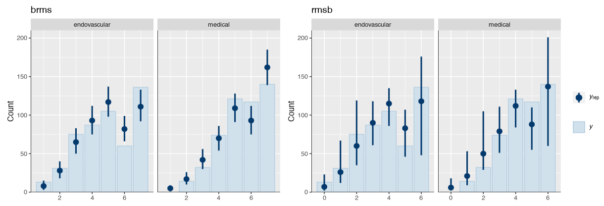
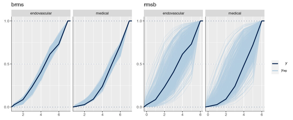
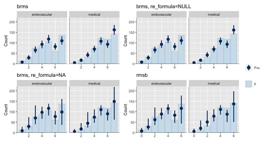
Is it possible that the pp_check implementation for the rmsb model is treating the random effects differently than the brms pp_check implementation when generating model predictions? For example, the code below reproduces your p1 and p2 plus two additional plots: p1a sets re_formula=NULL, which includes uncertainty due to random effect group levels, while p1b sets re_formula=NA which excludes uncertainty due to random effect levels. The re_formula argument is passed on to posterior_predict, and re_formula=NULL is the default. The plots are below, followed by the code.

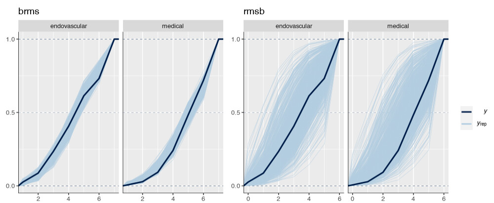
In the top row, the plot with an explicit re_formula=NULL is the same as the original brms plot, which is expected, given that the posterior_predict default is re_formula=NULL. In the bottom row, the plot of the brms model with re_formula=NA is similar to the plot generated from the rmsb model (though maybe this is just coincidental).

I’m actually confused by this. I expected the plot with re_formula=NULL to have wider uncertainty bands than the plot with re_formula=NA, because the former includes uncertainty due to varying levels of the random intercept while the latter does not. In any case, I thought I’d post this in case it has something to do with the differences you’re seeing between the two posterior checks.

p1 = pp_check(PO_brms, group = "x", type = "bars_grouped", ndraws = 1000) +
  labs(title = "brms") + coord_cartesian(ylim = c(0, 220))

p1a =  pp_check(PO_brms, group = "x", type = "bars_grouped", ndraws = 1000,
                re_formula=NULL) +
  labs(title = "brms, re_formula=NULL") + coord_cartesian(ylim = c(0, 220))

p1b = pp_check(PO_brms, group = "x", type = "bars_grouped", ndraws = 1000,
               re_formula=NA) +
  labs(title = "brms, re_formula=NA") + coord_cartesian(ylim = c(0, 220))

p2 = pp_check(PO_rmsb, group = "x", "bars_grouped", ndraws = 1000) +
  labs(title = "rmsb") + coord_cartesian(ylim = c(0, 220))

p1 + p1a + p1b + p2 + patchwork::plot_layout(guides = 'collect')
2 Likes

Based on my limited understanding, the rmsb Markov longitudinal models have no random effects. Accordingly, if specifying re_formula = NA ignores cluster-specific deviations of the intercept, it should produce pp_check plots similar to those produced by rmsb.

For those who are seeking to estimate group (“marginal”) effects in their analyses, the wide intervals in the pp_check plots should not deter them from using the incredibly useful rmsb package.

1 Like

Thanks Max. The problem in setting rsdsd = 0.01 is that it forces the rmsb model to be different from brms, which applies a scale parameter for the half t distribution for the SD of random effects = 2.5.

1 Like

Wow Joel, very nice!! And yes, I’d also expect opposite results with re_formula=NA. I will look this up in the Stan forum.

Honestly, I am not sure how predict.blrm handles random effects. Cc @f2harrell

Slightly better to say that Markov models usually do not need subject-level random effects because they handle within-subject correlation directly. But we can add random effects and see if we need them, which is one good way to check the first-order Markov assumption. Random effects assume a much different correlation pattern in which all previous Y’s are equally important in predicting the current Y, whereas first-order Markov states that you only need to know the most recent Y.

1 Like

But am I fitting a Markov longitudinal model?

Yong, can you please explain the rationale of this code snippet in your custom pp_check function?

pred_ordinal <- predict(modblrm, newdata, type="fitted.ind", posterior.summary = "all")
yrep_alldraws <-   apply(pred_ordinal, c(1,2), function (x) {
      myvec = unlist(rmultinom(1,1,x))
      myvec_names = modblrm$ylevels   ## get unique levels of Y
      return(myvec_names[myvec==1])
    })

I understand that predict(..., type = "fitted.ind") yields P(Y = {0, 1, 2, 3, 4, 5, 6} | X = newdata[x, study]).

Suggested nomenclature: Markov model vs. Markov model with random effects. Both are Markov models; the latter could be called an extended Markov model but let’s be explicit about random effects instead.

1 Like

Interesting. Can one say that predict.blrm() behaves like brms::posterior_epred(..., re_formula = NA) in Markov model with random effects?

As per brms documention:

re_formula formula containing group-level effects to be considered in the prediction. If NULL (default), include all group-level effects; if NA, include no group-level effects.

1 Like