Bayesian Regression Modeling Strategies

,

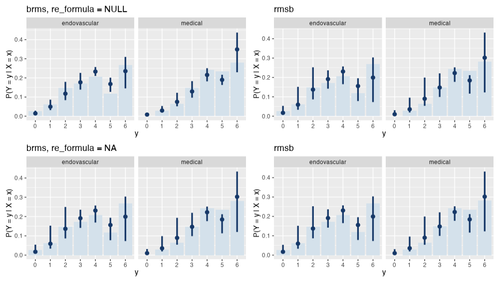
I was able to reproduce this behavior with brms::posterior_epred(..., re_formula = NA), which yields the same estimand as predict.blrm(). Note that the Y axis now represents P(Y = y | X = x) instead of Count.

nd = data.frame(x = c(rep("endovascular",3),
                      rep("medical", 3)),
                study = c("ANGEL-ASPECT", 
                          "RESCUE-Japan LIMIT",
                          "SELECT2")
)

# brms ---

brms_epred_NULL = 
  tidybayes::epred_draws(object = PO_brms,
            newdata = nd,
            re_formula = NULL,
            category = "mRS")

brms_epred_NA = 
  tidybayes::epred_draws(object = PO_brms,
                         newdata = nd,
                         re_formula = NA,
                         category = "mRS")

# rmsb ---

rmsb_epred = 
  predict(PO_rmsb,
          newdata = nd,
          type = "fitted.ind",
          # Extract all posterior draws:
          posterior.summary = "all") |> 
  posterior::as_draws_df() |> 
  dplyr::rename("data_id" = ".chain") |> 
  dplyr::as_tibble() |> 
  dplyr::mutate(
    x = dplyr::case_when(
      data_id == 1 ~ nd[1,"x"],
      data_id == 2 ~ nd[2,"x"],
      data_id == 3 ~ nd[3,"x"],
      data_id == 4 ~ nd[4,"x"],
      data_id == 5 ~ nd[5,"x"],
      data_id == 6 ~ nd[6,"x"]),
    
    study = dplyr::case_when(
      data_id == 1 ~ nd[1,"study"],
      data_id == 2 ~ nd[2,"study"],
      data_id == 3 ~ nd[3,"study"],
      data_id == 4 ~ nd[4,"study"],
      data_id == 5 ~ nd[5,"study"],
      data_id == 6 ~ nd[6,"study"]),
    ) |> 
  tidyr::pivot_longer(1:7) |> 
  dplyr::mutate(name = stringr::str_remove(name, "y=")) |>
  dplyr::rename("mRS" = name)


pd = 
  d |> 
  dplyr::group_by(x) |> 
  dplyr::count(y) |> 
  dplyr::mutate(p = n/sum(n))

p1 = 
  pd |> 
  ggplot() +
  geom_col(data = pd,
           aes(x = `y`, y = `p`),
           size = 2, fill = "#D4E1EB") +
  stat_pointinterval(data = brms_epred_NULL,
                     aes(x = mRS, y= .epred),
                     .width = 0.9,
                     color = "#163868") +
  labs(title = "brms, re_formula = NULL",
       y = "P(Y = y | X = x)") +
  facet_wrap(~x)

p2 = 
  pd |> 
  ggplot() +
  geom_col(data = pd,
           aes(x = `y`, y = `p`),
           size = 2, fill = "#D4E1EB") +
  stat_pointinterval(data = brms_epred_NA,
                     aes(x = mRS, y= .epred),
                     .width = 0.9,
                     color = "#163868") +
  labs(title = "brms, re_formula = NA",
       y = "P(Y = y | X = x)") +
  facet_wrap(~x)

p3 = 
  pd |> 
  ggplot() +
  geom_col(data = pd,
           aes(x = `y`, y = `p`),
           size = 2, fill = "#D4E1EB") +
  stat_pointinterval(data = rmsb_epred,
                     aes(x = mRS, y= value),
                     .width = 0.9,
                     color = "#163868") +
  labs(title = "rmsb",
       y = "P(Y = y | X = x)") +
  facet_wrap(~x)

(p1 + p3) / (p2 + p3)
3 Likes

@f2harrell, is there any way to get the estimand yielded by brms::posterior_epred(..., re_formula = NULL) but with predict.blrm() instead? i.e., to include “all group-level effects”

These codes generate the posterior predictive Y value by taking a random draw from a categorical distribution with an underlying vector of level probabilities. I wrote the function back in 2021 when I was trying my hands on using rmsb to analyze the “Bayesian logistic regression analysis” section in Prof Harrell’s bbr. The model doesn’t involve random effects.

1 Like

@arthur_albuquerque For my own understanding and learning, could you kindly explain why you have used tidybayes::epred_draws - and not tidybayes::predicted_draws - in your recent post? I asked because in an earlier post, you mentioned that brms::pp_check() uses brms::posterior_predict().

Thank you in advance for your clarification.

1 Like

Because I wanted to compare epred_draws(..., re_formula = NA)'s output with predict.blrm’s. Both yield the same estimand.

1 Like

Thank you for the clarification! Again, for my own learning, do you know how brms::posterior_predict(re_formula = NULL) incorporates group-level effects? I ask because I have tried - but failed - to comprehend its inner workings.

If you do, and for what it is worth, PO_rmsb$gammas and ranef(PO_brms) seem to generate fairly similar results (which is assuring!) and I thought they might assist you in your quest to generate pp_check plots for blrm models.

> PO_rmsb$gammas
gamma[1] gamma[2] gamma[3] 
 -0.2556   0.2204   0.4643 
> ranef(PO_brms)
$study
, , Intercept

                   Estimate Est.Error   Q2.5 Q97.5
ANGEL-ASPECT        -0.1722    0.5066 -1.008 1.085
RESCUE-Japan LIMIT   0.3001    0.5135 -0.519 1.569
SELECT2              0.5526    0.5178 -0.264 1.837

1 Like

No :sweat_smile:

I found this explanation here:

I suspect that it predicts the global grand mean and then adds the random effect to each group represented by the random intercept.

Edit: Yes, sounds like it. On the other hand, re_formula = NA omits the random effect from the computation. @f2harrell can you please confirm that predict.blrm() also omits it?

1 Like

This will make me look foolish but as a first attempt, I have tried to incorporate the random effects by doing the following:
(i) Extract the random effects and antilog them to create ORs
(ii) Use the nifty Hmisc::pomodm function to shift the level probabilities by the ORs
(iii) Use the rmultinom() function to take random draws from a categorial distribution with the new (shifted) level(cell) probabilities
(iv) Use the pp_check() function to generate the resultant plots

I’m not fully certain, but this (failed) method seems to produce point estimates that are closer to those by brms. Of course, the intervals remain wide, and I would appreciate any guidance and suggestions on where I have gone wrong.

As an aside, Step (ii) using the for-loop resulted in a time-consuming process and I would appreciate guidance on how I can write more efficient codes.

Many thanks to all!

pred_ordinal <-   predict(PO_rmsb, type = "fitted.ind", posterior.summary = "all") 
myor <- exp(PO_rmsb$gammas)  ## extract RE, antilog values to convert to ORs
names(myor) <- levels (as.factor(d$study)) 
myor1 <- myor[d$study]


#' Shift the level probs by RE-based ORs using the nifty Hmisc::pomodm 
#' (painfully) slow process (there must be a faster way to do this!)
for (i in 1:nrow(d))  
  for (j in 1:4000) {
    pred_ordinal[j,i, ] <- pomodm( p = pred_ordinal[ j, i, ], odds.ratio = myor1[i]  )
  }
 

#' take random draws from categorical distribution with the adjusted level probs
yrep_alldraws <-   
  apply(pred_ordinal, c(1,2), function (x) {
    myvec = unlist(rmultinom(1,1,x))
    myvec_names = PO_rmsb$ylevels    
    return(myvec_names[myvec==1])
  })
yrep_alldraws <- apply(yrep_alldraws, c(1,2), as.numeric) 
yrep          <- yrep_alldraws[c(1:4000), ]

y <- d [ , all.vars(PO_rmsb$sformula)[1] ] 
y <- as.numeric(as.character(y))
ppc_args <- list(array(y), yrep)
ppc_args$group <- d[["x"]]

p_rmsb <- 
  do.call(bayesplot::ppc_bars_grouped, ppc_args) +
  labs(title = "rmsb, my first + failed attempt") + coord_cartesian(ylim = c(0, 220))

p_brms <-
  pp_check(PO_brms, group = "x", type = "bars_grouped", ndraws = 1000, re_formula=NULL) +
  labs(title = "brms, re_formula=NULL") + coord_cartesian(ylim = c(0, 220))

p_rmsb + p_brms + patchwork::plot_layout(guides = 'collect')


1 Like

Hi all

I am running a partial proportional odds model that has some divergent transitions. I was wondering if it is possible to change the target acceptance probability rate (adapt_delta) directly using the blrm command to address this?

Are you using rstan (the default), or cmdstan?

I am currently using rstan.

Please try passing the extra arguments you need to rstan::sampling to blrm and let me know what you get.

Thanks for your response. When running the following model, I’ve tried to use the argument from rstan::sampling (the control argument):

ppomod <- blrm(y~x,ppo = ~x, priorsd = 5, priorsdppo = 5,
              conc = 1, seed = 10993, iter=6000, chains=4,
              control=list(adapt_delta = 0.9))

This then gives the following error:

Error: passing unknown arguments: control.

Sorry about that. In the next release of rmsb I’ll add an argument samplingArgs or sampling_args that will allow you to specify a list of arguments to pass to rstan::sampling() or the equivalent with cmdstan.

But I recommend you switch to cmdstan with rmsb in the meantime as it has better sampling performance and is faster.

2 Likes

Thanks Frank, that’s really appreciated! It would also be great to include the user to specify the maximum tree depth as well when divergent transitions arise (control=list(max_treedepth=x) in rstan).

When are you planning on releasing the next version of rmsb? :slight_smile:

1 Like

I am a medical researcher doing mostly population-based epidemiological studies, prospective cohort studies and (soon) pragmatic randomised controlled trials. Over the next couple of years, I want to move over to a fully Bayesian approach - I am convinced that this is a more reasonable theoretical framework. One of the big sticking points for me is that I “know how to write” a concise medical journal article using “standard statistical terminology”. I know what editors, reviewers and the general medical readership expect and where they expect to find it. I know what they will understand and accept. I have trouble imagining how I would write a fully Bayesian publication. Where and how do I provide information on the priors? How do I report credible intervals or probabilities? My worry is that most Bayesian studies I have read have been very technical, long and fairly dense and outside of medical journals I and my peers normally read. I was hoping someone could point me to examples of fully Bayesian analyses published in main-stream medical journals that were particularly well reported so I can use these as case-studies in how I would write up a Bayesian study and to convince my co-authors of adopting this approach.

2 Likes

I’m hoping for July 15.

Let’s work at compiling such a list. I have a small collection of published clinical trials using Bayes and need to generalize that. This paper has some pieces of the reporting puzzle. I think we could also create a topic on datamethods for crowdsourcing a template for Bayesian results reporting.

2 Likes

Thanks Frank. Just wondering if there is any update on a release date? :slight_smile:

Sorry I got behind. I’ll start working on it again and will keep you posted.

1 Like

Which operating system are you running? If Mac is it post-2020 Mac or pre-2020 Mac?