Good morning, I wanted to ask about the similarities and differences of the subgroup analysis, between frequentist versus Bayesian statistics. As far as I know, for a frequentist model the term interaction is introduced in the formula, for example survival ~ treatment + histology + treatment * histology + x1 + x2 …
After that you calculate the therapeutic effect in each group according to histology, and the P value of the interaction term is useful to assess whether the effect is different or not in both strata. I have doubts to understand how this is done with a Bayesian approach.
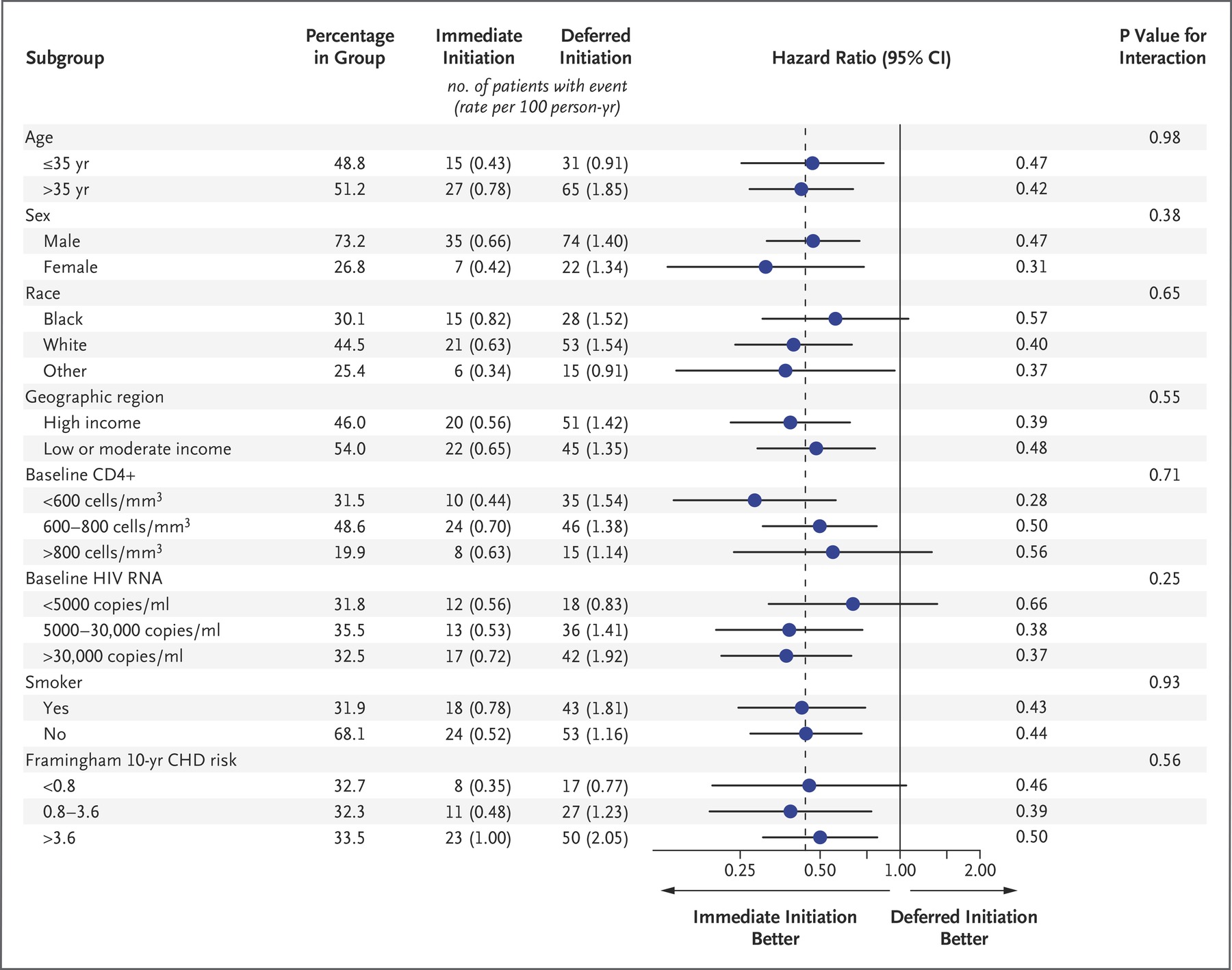
I have thought that one option is to make it similar to the frequentist approach, as in the attached figure, drawing the credibility intervals, and changing the P-value for interaction with Bayes factors. However, I don’t know if there is any other specific method to do this.
Second question: although it is not a specific Bayesian problem, I wanted to ask you what is the best strategy to perform a subgroup analysis similar to the one in the figure. Should all interactions be entered at once, or one by one at each step? Is it a good idea to adjust for the issue of multiple comparisons?
Thanks.
Bayesian model averaging is an appealing approach since you can place priors directly on the probability that an interaction is included and then you get mode uncertainty incorporated in your estimates automatically. A simple toy example in JAGS for a binomial outcome could be something like:
Monitoring in.mod would give you the probability that a variable is selected. An approach I have seen at times is to run this on all variables, exclude the ones with negligible posterior probabilities and then run again on your limited set.
All the same dangers of bayes factors exist here though, i.e. posterior inclusion probability will be sensitive to priors on parameters even though the parameters themselves might not be. See https://arxiv.org/pdf/1704.02030.pdf for a discussion of alternatives which have been implemented in rstanarm/brms.
Note that the table presented at the top contains improper analysis. Effects are not covariate adjusted, and continuous interacting variables are arbitrarily categorized.
To me it is best not to think of the interaction being “in” or “out” but rather to carefully elicit priors for the magnitude of interaction effects. This is the central theme of Simon R and Freedman LS. 1997. Bayesian design and analysis of 2 by 2 factorial clinical trials. Biometrics 53:456-464.
Even though the model should be saturated with regard to main effects, the question remains about whether the interactions should be adjusted for each other. I lean towards analyzing the interactions separately because of collinearity. I discuss this in BBR Section 13.6.
More or less, I think I understand the subtleties of BBR. I was wondering if it would be a good idea to use the rms capabilities, both the contrast function and the graphs, to analyze the study with a frequentist approach, as described in the notes, and then do another Bayesian analysis as a complimentary analysis, in the same article (to report posterior probabilities under the prior).
I wanted to analyze the effect of a new type of chemotherapy on gastric cancer. There is a previous clinical trial, with an HR 0.77, 95% CI, 0.65-0.99. I could give more details if someone is interested, for now better leave it simple.
I have an observational registry with n > 1500 and I would like to assess if this main effects differs according to some factors (mainly histology). I suspect that might happen and nobody has checked before.
The formula to use for main effects would be something like this: cph (surv ~ new_treat + histology + rcs(age) + rcs(year)
Then for interactions one by one, new_treat * histology, etc. would be introduced. And I use the contrast function.
The notes start with the phrase “Anything resembling subgroup analysis should be avoided”, then I no longer dare to present a subgroup effects table, but I will show the graphs after applying the contrast function, as in the examples. In addition to histology, other interactions could be with tumor extent, age and year of treatment (four in total).
For the Bayesian part I had thought to use this previous knowledge in the literature (HR 0.77) as a prior of the main therapeutic effect. After that I wanted to analyze the effect according to histology, since I have good reasons to think that not all histological types respond equally to treatment. To model the interaction in the bayesian model I could use a relatively skeptical prior (for the interaction term), and report the posterior probability that the new treatment is superior to each group according to histology. But this could be done in parallel to the frequentist analysis, to use the full power of the rms package.
There are two things about BBR notes that I don’t understand.
Need to use penalized estimation (e.g., interaction effects as random effects) to get sufficient precision of differential treatment effects, if # interaction d.f. > 4
I don’t know how to apply this.
I also don’t understand the chunk test with all potential interaction R effects combined. I don’t know how this would be done.
Without time to go into detail, this is pretty reasonable. But the frequentist approach you suggested has these disadvantages:
Testing treatment effect and then testing an interaction effect, using two different models, is often done but does distort the operating characteristics of the tests.
The approach requires a huge sample size or an acknowledgement of inadequate power, so that only mammoth interactions are likely to be detected.
The combine-all-interactions chunk test is automatically produced by rms::anova.
Formatting suggestion: enclose inline code in backticks.
Two doubts that stem from this answer would be the following:
In another post in Datamethods it has been commented that the correct way to analyze interactions could be with the contrast function of rms. For example,
fit<-cph(sur~ treat+treat*sex , data=data,x=TRUE , y=TRUE)
sex <- 0:1
c<- contrast(fit, list(treat=1,sex=sex),
             list(treat=0, sex=sex))
c
However, as a contrast, I would find it interesting to compare the mathematical difference between this method and the use of subset. For example:
Secondly, I would like to know how the effect of treat could be estimated through the first model (fit), regardless of the interaction (average unconditional effect), in order to obtain the same as in:
fit4<-cph(sur~ treat, data=data,x=TRUE , y=TRUE)
Sorry to everybody if these questions are very easy or trivial.
Models with sex in them won’t fit if you subset on sex. Fit a single model and do the needed contrasts—both the sex-specific treatment contrasts and any double difference contrasts to estimate interaction effects (you can give contrast four lists A B C D and it will compute (A-B) - (C-D).
Only with ordinary linear models are those two results the same for the point contrast estimate (they yield difference variances however). For the Cox PH model, using sex as a covariate assumes PH for sex, and this will yield a different point estimate for treatment than the model that stratifies on sex and doesn’t assume PH for it.
I assume you’re discussing a randomized study so that the moderators are orthogocal to treatment. Then the main problem is the moderators may not be orthogonal to each other. Things get tricky and I often recommend running two separate models. But we need a more general approach. What is the rank correlation between the two moderators?