This is a topic for questions, answers, and discussions about session 16 of the Biostatistics for Biomedical Research course for 2020-04-24. Session topics and links are listed here . The session covers transforming variables, measuring change, problems with change scores, and regression to the mean.
I have a question about the change of exposure. Is it the same strategy as the change of the outcome? If I want to evaluate the change of ordinal exposure, the right way to model it should be:
Assume Y is the outcome and X is the exposure (without considering covariates), then
library (rms)
ols (Y~pol(Xbaseline, 2)+pol(Xfollow-up, 2))
I am wondering whether it is the right way to think about this issue.
It is simple to think about this if you have two baseline measures (say one historical one and one measurement just as follow-up starts). But if your Xfollow-up is measured at the same time as Y this gets harder to interpret. It’s then a cross-correlation analysis, and you might find some good thinking about that in the econometrics literature.
1 Like
Thank you so much, Frank!
You really got my point which I initially had a rough idea.
It is the actual situation I encountered. Xfollow-up was measured at the same time as Y. But the good thing is I have only one Xhistorical, not several. It seems I could handle it through a simple way rather than a cross-correlation analysis.
Not sure. The fact that you will be analyzing Xfollow-up means that cross-correlation analysis is what you are doing.
1 Like
Hi @f2harrell ,
I watched the YouTube video on this session, and I am interested in the topic discussed towards the end (40:37min BBR16: Biostatistics for Biomedical Research Session 16 - YouTube).
If I understood correctly, you suggest fitting a model with multiple time points as:
y1 + y2 + … + yk ~ y0 + treatment
You mentioned in the video that further explanations could be found in the RMS’ Course Notes. Yet, I wasn’t able to find notes on this topic in specific.
Could you provide further references on this type of modeling? I would love to delve into it.
Thank you!
Please see the Modeling Longitudinal Responses chapter in the RMS course notes. At the end of that chapter you’ll see new material about Markov longitudinal models, which are quite flexible.
Thank you for the quick reply. I will definitely take a look.
Dear Professor @f2harrell,
I’m using the suggested routine/code provided in Chapter 14 of BBR for analyzing a randomized two-group parallel design (simulation study). After fitting the semiparametric ANCOVA/proportional odds model, how can I get the 0.95 confidence interval for the ‘group’ coefficient? Is there an example (with the code) in BBR or RMS on how I can use bootstrap in a situation like this to obtain a more reliable estimate of the treatment effect? I’m also ploting the predicted means from the model.
Note: I’m assuming there’s no interaction between baseline scores and group, i.e., that the treatment effect is independent of the baseline scores.
Thank you.
The central treatment parameter is the treatment group indicator’s odds ratio. This may be able to be converted into a concordance probability (the conversions almost exact if there are not covariates) but the OR stands on its own and is interpreted along these lines: The treatment B:A OR is the ratio of odds that Y \geq y for treatment B divided by the odds that Y \geq y for A, for any y other than the lowest level of Y.
For more clinical interpretation you can also compute covariate-specific differences in mean (if Y is interval-scaled) or median (if Y is continuous). Getting confidence intervals for those is difficult, but p-values for OR applies to them also.
Thank you.
Looks like I can get the answer I’m looking for by simply passing the fitted model through summary(). Is that correct? Please see attached image.
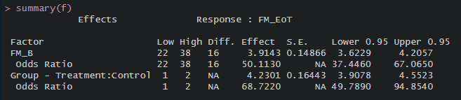
The reason I ask is because I simulated a treatment effect such that subjects in the treatment group score 5 points higher on the FM scale (0-66) than subjects in the control group at the end of the intervention. The simulated sample size is 1000. The obtained coefficient for ‘group’ is 4.23 [95%CI(3.90 - 4.55)]. The OR is 68.72 [95%CI(49.79 - 94.85)].
The question is: The metrics I should use for concluding that the analysis was performed correctly (in keeping with what was simulated) is the ‘group’ coefficient of 4.23 [95%CI(3.90 - 4.55)], correct? Also, is the fact that the estimated CI does not include the simulated effect (+5) due simply to sampling variability? That’s why I also asked about the bootstrap…
Thank you again.
Have you tried the R package marginaleffects? It supports rms models
The package provides a few methods for the 95% CI, such as the delta method and bootstrapping
1 Like
I’ve heard of this package.
Will check it out.
Many thanks!
I’d worry about an instability caused by a too-small sample size. Please give a frequency tabulation of group x the outcome variable.
Your other variable also has a huge odds ratio. I donl’t really trust your simulation setup as I seldom see effects that huge.
I see. I have another question then:
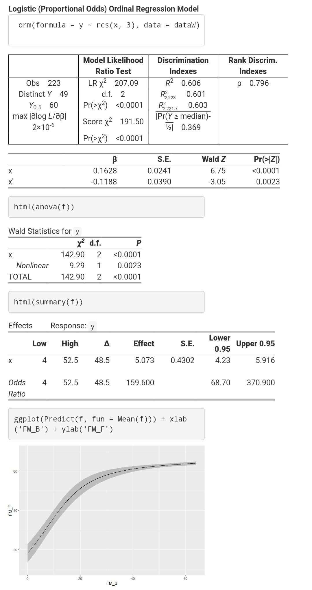
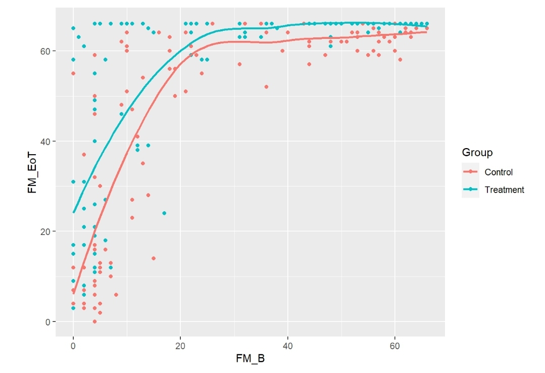
Now using real data from 220 patients who were assessed 1 week after their stroke (baseline,
FM_B) and then after 6 months (follow up, FM_F). FM is a motor recovery scale ranging from 0 to 66
(the highest the better). No specific intervention was given to these patients besides usual care.
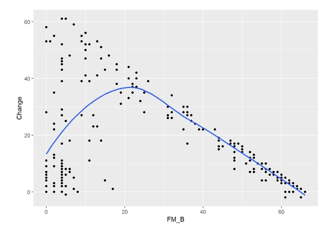
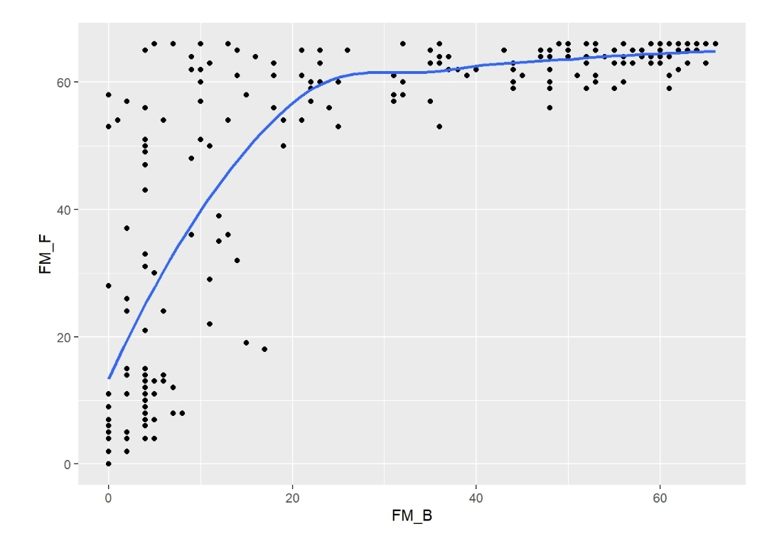
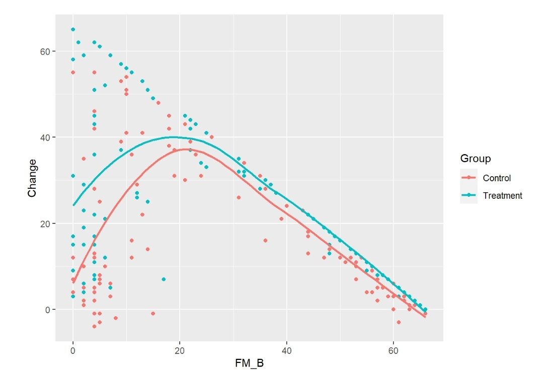
There’s a rather nonlinear association between FM_B and FM_F, and between FM_B and Change
(FM_F minus FM_B) (Figures). The association between FM_B and FM_F was tested with a
Logistic Ordinal Regression Model. There’s a strong association: p-value from 2df test from anova <0.0001; OR from summary = 159.6 [95%CI (68.7 - 370.9)).
This OR is huge, showing that baseline motor status is a strong predictor of motor status at 6 months. What’s wrong with that?
Thank you.
Nothing wrong with that. You’d expect baseline function to be a dominant predictor; I’m not used to it being that dominant but there is nothing wrong with the analysis.
1 Like
Many thanks, Professor.
Following up on this issue,
Using the simstudy package, I randomly assigned those 223 patients from above to either Treatment or Control (Group covariate).
Then, I added 5 points to the FM_F scores from those in the Treatment group, using the following formula:
‘FM_EoT = FM_F + 5 * Group’, with a variance of 4 and where:
‘EoT = End of Treatment’
‘FM_F = follow up score from the real data’
‘Control coded as 0’
‘Treatment coded as 1’
See attached figures.
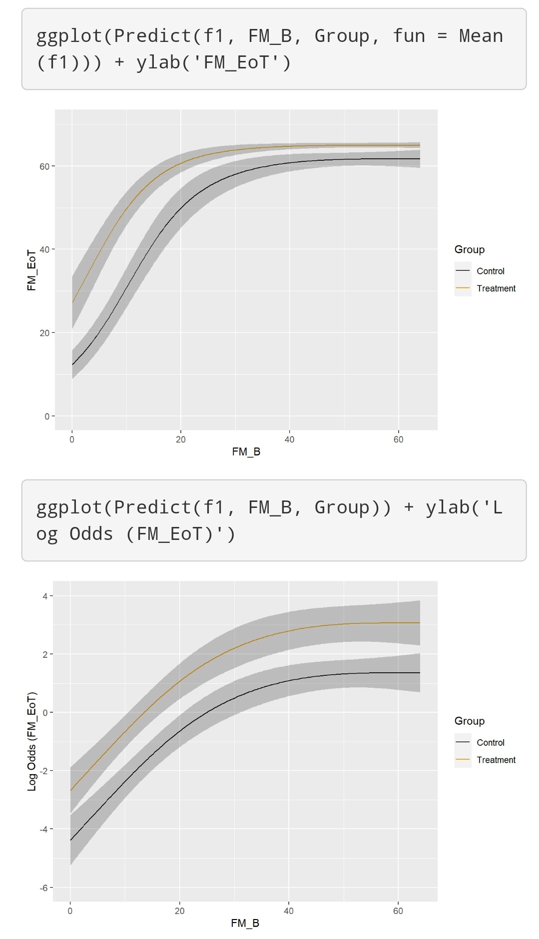
Finally, I tested the effect of my simulated intervention with a Semiparametric ANCOVA using again a Logistic Ordinal Regression Model:
FM_EoT ~ rcs(FM_B, 3) + Group
All tests from the anova were <0.0001 and the ORs from summary were 135 [95%CI (59.65 - 305.4)] for FM_B, and 5.5 [95%CI (3.27 - 9.35)] for Group. The effect plots are also attached.
My goal is to test different analysis approaches (semiparametric vs parametric ANCOVA, using
change from baseline, etc).
How do I know which analysis approach will be the best/more correct? I think the one that most closely replicates the simulated effect, right? How does the Group OR from the above analysis relate to my simulated treatment effect?
Should I use bootstrap to compensate for the small sample size (223) and get a more reliable estimate? If yes, how? I tried bootcov and then summary but it doesn’t seem to work.
Thank you.
It appears that you are using an additive model to do simulations instead of using a true proportional odds model. There is also a chance that you are not incorporating the needed uncertainties in generating the data (in the additive linear model this amounts to not adding residuals that are large enough), resulting in unrealistically extreme significance.
Frank, thanks for the amazing content in the BBR sessions. I am a late-comer but found them very informative and useful.
I have two questions:
- I typically work with weight loss data and the clinical standard for this is percent weight loss. I was wondering if you have any experience working with this and what suggestions you may have since it is not the ideal way to analyze the data (i.e. measuring outcome with baseline as a covariate)?
- I have seen conflicting literature with using the baseline as a covariate in non-randomized trials (Lord’s paradox). It seems to me like whether or not it introduces bias depends on the specific question and DAG. Is this correct?
That’s correct and I don’t have enough experience with that in observational studies. Speaking in general I think that percent weight lost would not be correct because weight loss is probably somewhere between absolute and relative. I would take absolute weight as the outcome adjusted for a flexible function of baseline weight.
1 Like