This is a place for questions, answers, and discussion about session 8 of the Biostatistics for Biomedical Research airing 2020-01-03 and dealing with study design and comparing two proportions and introducing logistic regression to do so. Session topics are listed here. The video will be in the YouTube BBRcourse Channel and will be directly available here after the broadcast.
The session covers reasons why not to use Fisher’s “exact” test.
I don’t have plans to cover those. For the future I’d like pointers to a literature that covers covariate-specific counterparts to those. The course focuses on clinical and pre-clinical biostatistics and not population health.
-i’d say the speed of pearson is not a deciding factor, unless eg you have a macro to produce a standard table 1 and there’s a risk that the user mispecifies a continuous variable in the macro call, then fisher will cause sas to hang rather than simply fail, or if you’re doing simulations eg for power estimation and have to run fisher thousands of times, although i’ve done that before in sas and it wasn’t so bad (incidentally, I ran exact wilcoxon in proc npar1way recently and it hangs, i’d avoid it for any reasonable n)
-regarding the conservative p-value, this might be an argument for, rather than against eg in a standrad table 1 with many dichotomous patient characteristics (presence/absence of conditions), if the client demands p-values it may be a cautious (ie devious) way for the statistician to discourage the client from overreacting to pvals?
-regarding conditioning on the number of events, you persauded me on bayes. I checked the statsexchange link and one of the SiM papers and they don’t mention the bayes option. I found this paper: Comparison of Three Calculation Methods for aBayesian Inference of P(π1 > π2). They suggest the exact method is difficult to implement in sas and suggest mcmc method instead
Oddly enough in GWAS it is common to use Fisher’s test. Not only is it less accurate, it poses a significant computational burden with large numbers of subjects and huge numbers of candidate SNPs.
I’d rather that p-values and type I error probabilities mean what they say, and that if you want to be conservative you incorporate methods that bring conservatism in at the right point in the logic flow. That would be for example using Bayesian shrinkage priors such as the horseshoe prior (second best is probably elastic net). Alternatively, a frequentist might elect to do a multiplicity adjustment on p-values from a series of Pearson \chi^2 tests.
i know how it sounds, but if the artificial inflation was made too explicit then the client might object. Poor biostat consultants are doomed to become cynics
it’s done all the time though, ppl know bonferroni is conservative but still use it, it’s a mild confession that we do not have complete faith in p-values + we’re more fearful of t1 errors than t2. Aside: in dealing with clients i’ve found that the technical argument never wins, never ever, one must instead say: the regulator/reviewer will lose confidence in you, then you have them
But the point is that using Bonferroni is transparent. The use of Fisher’s “exact” test to achieve conservatism is very non-transparent and represents slight-of-hand.
But know that the use of any multiplicity adjustment should be questioned. You can virtually abolish increases in type I error probabilities by testing against nonzero values. Even better: do a simple likelihood ratio for odds ratio = 1.2 against odds ratio of 2.5. Increases power while simultaneously controlling type I error.
i meant bonferroni is more conservative than intended ie if tests are correlated, and that this is usually understood by the stato and not understood by the non-stato, even when the stato attempts to explain it, they still want it, and maybe the stato resigns themselves to this because it’s conservative.
eg’s are too numerous, eg locf was used when we new it was biased, but it was biased in the ‘right’ direction, i explained this to a client and they wanted it anyway because it’s what everyone was doing. you’d only win the argument by suggesting the reviewer/regulator would not like it
re your 2nd point: i’m looking at a sap at the moment with bonferroni correction, and wondering how to escape it. The outcome is a on a scale where it’s not easy to specify a non-zero value for the null. I might suggest a composite …
Watched this session today. Any good references on comparison of Fisher’s Exact Test and the ordinary Pearson chi-square as well as discussion on the need of Yates’ correction?
It’s something that as a reviewer would be useful as lots of papers I review just use the standard: “As expected frequencies were < 5, FET was used”
Yes this is a common question. The original idea of < 5 was made up by Pearson or Cochran, without checking it. He was wrong. Great discussions about this are on stats.stackexchange.com although I’ve forgotten the best page there. See also https://en.wikipedia.org/wiki/Fisher’s_exact_test
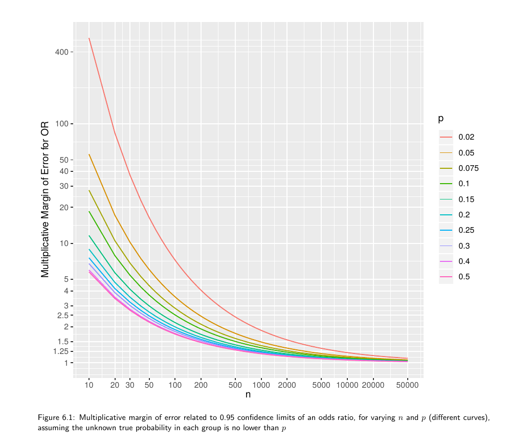
I keep seeing the videos a little late. I didn’t quite understand the multiplicative margin of error. Can someone clarify the concept for me in a simple way? Thank you.
In estimating means we often thinking of a margin of error as twice the standard error of the mean. Replace the “2” with “1.96” or an appropriate critical value and you have margin of error = half width of a 0.95 confidence interval.
Now think of a quantity where a ratio is the appropriate effect measure, e.g., odds ratio, hazard ratio. The confidence interval should always be constructed on the log scale (unless using the excellent profile likelihood interval which is transformation-invariant). We compute the margin of error on the log ratio scale just as we did for the mean above. This is 1/2 of the width of the confidence interval for the log ratio. If you antilog that margin of error you get the multiplicative factor, i.e., the multiplicative margin of error. Suppose that the MMOE is 1.5. This means that you can get the 0.95 confidence interval for the ratio by taking the ratio’s point estimate and dividing it by 1.5 and then multiplying it by 1.5. You can loosely say that our point estimate can easily be off by a factor of 1.5.
So if I was planning a pilot study and the hypothetical odds ratio was 2, with a MMOE=1.5 in the statistical plan, I could obtain the sample size for that trial with a given precision, such as the 95% confidence interval for that odds ratio was 2/1.5 for the lower limit, and 2*1.5 for the upper limit. Right?