Sorry if this is an elementary question. I was tasked with analyzing repeated measures of protein expression (baseline and 6-month follow-up; 2 time points so far) across two treatment groups (44 subjects, 357 features). The goal was to identify differentially expressed proteins for the following contrasts:
- group A at baseline vs group A at 6 months
- group B at baseline vs group B at 6 months
- group A at baseline vs group B at 6 months
- group B at baseline vs group A at 6 months
- group A vs group B at baseline
- group A vs group B at 6 months
I was asked to validate our customer’s analysis, which involved t-tests for the contrasts above, and to suggest alternative approaches. I used three modeling strategies:
- Unpaired t tests (customer’s approach)
- Paired t tests where appropriate
- linear mixed model: y ~ treatment*time + age + (1|subject_id)
For each contrast and modeling strategy, I obtained a list of differentially expressed proteins.
Inspired by this post by Prof. Harrell, I decided to assess the stability of protein rankings using bootstrap resampling. I would appreciate feedback on my bootstrapping code from more experienced statisticians.
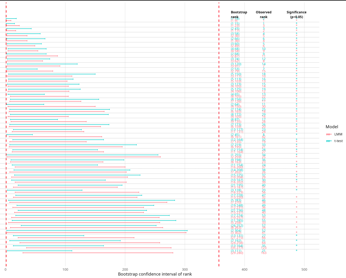
The bootstrapped confidence intervals for ranks from the linear mixed model are consistently wider than those from the t-tests (1,000 bootstraps). My interpretation is that the t-tests may produce overly confident rankings, as they do not account for the effects of age and time, the effect of the interaction between time and treatment, and the effect of within-subject variation.
Does this interpretation sound reasonable? Shown is a plot for the same contrast for each modelling strategy.
Code for bootstrapping of the t-tests:
run_bootstrap_rank_ci <- function(data,
                                  contrasts,
                                  results_all_ttest,
                                  n_boot = 100, output_dir) {


  all_boot_ranks <- list()

  for (name in names(contrasts)) {
    contrast <- contrasts[[name]]
    message("Running bootstrap for contrast: ", name)

    data_filtered <- data %>% filter(eval(contrast$filter))


    observed <- results_all_ttest %>%
      filter(contrast == name) %>%
      mutate(
        abs_statistic = abs(statistic),
        observed_rank = rank(-abs_statistic, ties.method = "average"),
        direction = ifelse(estimate > 0, "Positive", "Negative"),
        test_type = case_when(
          method == "Paired t-test" ~ "paired_ttest",
          method == "Welch Two Sample t-test" ~ "unpaired_ttest",
          TRUE ~ "unknown"
        )
      ) %>%
      select(OlinkID, Assay, Adjusted_pval, statistic, observed_rank, direction, test_type)

    test_type_unique <- unique(observed$test_type)
    if (length(test_type_unique) != 1) {
      stop("Ambiguous or mixed test types detected for contrast: ", name)
    }

    test_type <- test_type_unique

    boot_ranks <- future_map(1:n_boot, function(i) {
      message("Bootstrap #", i)

      subject_ids <- unique(data_filtered$SubjectID)
      resampled_ids <- sample(subject_ids, size = length(subject_ids), replace = TRUE)

      boot_data <- map2_dfr(resampled_ids, seq_along(resampled_ids), ~ {
        subj_data <- data_filtered %>% filter(SubjectID == .x)
        if (nrow(subj_data) == 0) return(NULL)
        subj_data %>%
          mutate(SubjectID = paste0(SubjectID, "_boot", .y),
                 SampleID = paste0(SampleID, "_boot", .y))
      })

      boot_result <- if (test_type == "paired_ttest") {
        olink_ttest(df = boot_data, variable = contrast$variable, pair_id = "SubjectID")
      } else {
        olink_ttest(df = boot_data, variable = contrast$variable)
      }

      boot_result %>%
        select(OlinkID, statistic) %>%
        mutate(rank = rank(-abs(statistic), ties.method = "average"))
    }, .options = furrr_options(seed = TRUE))


    all_ranks <- bind_rows(boot_ranks, .id = "bootstrap_id")
    rank_ci <- all_ranks %>%
      group_by(OlinkID) %>%
      summarise(
        rank_0.025 = quantile(rank, 0.025, na.rm = TRUE),
        rank_0.975 = quantile(rank, 0.975, na.rm = TRUE),
        .groups = "drop"
      )


    annotated_results <- observed %>%
      left_join(rank_ci, by = "OlinkID") %>%
      mutate(
        rank_annotation = paste0("(", round(rank_0.025), " ", round(rank_0.975), ")"),
        label = paste0(
          rank_annotation, ", Rank: ", round(observed_rank),
          ", p = ", signif(Adjusted_pval, 2)
        )
      ) %>%
      arrange(observed_rank)

    all_boot_ranks[[name]] <- annotated_results
  }

  final_results <- purrr::map_dfr(names(all_boot_ranks), function(key) {
    # Retrieve the current data frame
    df <- all_boot_ranks[[key]]

    # Add the key as a new column
    df$contrast <- key

    return(df)
  })
  final_results <- bind_rows(final_results)

  write.csv(final_results,
            file = file.path(output_dir,"bootstrap_rank_summary.csv"),
            row.names = FALSE)

  return(final_results)
}
Code for bootstrapping of the linear mixed model:
run_bootstrap_lmer_posthoc <- function(original_data,
                                       original_posthoc_results,
                                       n_boot = 100,
                                       output_dir,
                                       variables = c("Time..months.", "Medication"),
                                       random_effects = c("SubjectID"),
                                       covariates = "Age.started.therapy",
                                       interaction_term = "Time..months.:Medication") {

  required_cols <- c("OlinkID", "Assay", "estimate", "Adjusted_pval", "contrast")
  missing_cols <- setdiff(required_cols, colnames(original_posthoc_results))
  if (length(missing_cols) > 0) {
    stop("Missing required columns in original_posthoc_results: ", paste(missing_cols, collapse = ", "))
  }


  observed_posthoc <- original_posthoc_results %>%
    dplyr::mutate(
      abs_estimate = abs(Adjusted_pval),
      direction = ifelse(estimate > 0, "Positive", "Negative")
    ) %>%
    dplyr::group_by(contrast) %>%
    dplyr::mutate(observed_rank = rank(abs_estimate, ties.method = "average")) %>%
    dplyr::ungroup() %>%
    dplyr::select(OlinkID, Assay, estimate, Adjusted_pval, contrast, observed_rank, direction)


  boot_ranks <- furrr::future_map(1:n_boot, function(i) {
    message("Bootstrap replicate: ", i)

    subject_ids <- unique(original_data$SubjectID)
    resampled_ids <- sample(subject_ids, size = length(subject_ids), replace = TRUE)

    boot_data <- purrr::map2_dfr(resampled_ids, seq_along(resampled_ids), ~ {
      subj_data <- original_data %>% dplyr::filter(SubjectID == .x)
      if (nrow(subj_data) == 0) return(NULL)
      subj_data %>%
        dplyr::mutate(
          SubjectID = paste0(SubjectID, "_boot", .y),
          SampleID = paste0(SampleID, "_boot", .y)
        )
    })

    # Fit LMER model
    lmer_results_lm_boot <- olink_lmer(
      df = boot_data,
      variable = variables,
      random = random_effects,
      covariates = covariates
    )

    lmer_results_twoway_significant_boot <- lmer_results_lm_boot %>%
      dplyr::filter(term == interaction_term) %>%
      dplyr::pull(OlinkID)

    # Post-hoc
    posthoc_boot <- olink_lmer_posthoc(
      df = boot_data,
      olinkid_list = lmer_results_twoway_significant_boot,
      variable = variables,
      random = random_effects,
      covariates = covariates,
      effect = interaction_term
    )

    posthoc_boot %>%
      dplyr::mutate(abs_estimate = abs(Adjusted_pval)) %>%
      dplyr::group_by(contrast) %>%
      dplyr::mutate(rank = rank(Adjusted_pval, ties.method = "average")) %>%
      dplyr::ungroup() %>%
      dplyr::select(OlinkID, contrast, rank)
  }, .options = furrr::furrr_options(seed = TRUE))

  all_ranks <- dplyr::bind_rows(boot_ranks, .id = "bootstrap_id")


  rank_ci <- all_ranks %>%
    dplyr::group_by(OlinkID, contrast) %>%
    dplyr::summarise(
      rank_0.025 = quantile(rank, 0.025, na.rm = TRUE),
      rank_0.975 = quantile(rank, 0.975, na.rm = TRUE),
      .groups = "drop"
    )


  annotated_results <- observed_posthoc %>%
    dplyr::left_join(rank_ci, by = c("OlinkID", "contrast")) %>%
    dplyr::mutate(
      rank_annotation = paste0("(", round(rank_0.025), " ", round(rank_0.975), ")"),
      label = paste0(
        rank_annotation,
        ", Rank: ", round(observed_rank),
        ", p = ", signif(Adjusted_pval, 2)
      )
    ) %>%
    dplyr::arrange(contrast, observed_rank)


  readr::write_csv(annotated_results, file.path(output_dir, "bootstrap_rank_summary.csv"))

  return(annotated_results)
}