Hello everyone,
One question that often comes up is whether a model/variable provides consistent levels of risk-discrimination across various subgroups of interest* (e.g., by sex, race, or other similar variables typically analyzed in a categorical fashion). This is straightforward to tackle by using interaction terms (if necessary) and calculating C-statistics in these subgroups.
When this is desired for continuous variables (e.g., age), the typical approach is to categorize the variable in some manner (e.g., <65 and >=65) and compare C-statistics in these subgroups. The problem with this is the arbitrary nature of dichotomization, its susceptibility to manipulation (using the “right” cutoff resulting in the desired outcome), and statistical imprecision/wider CIs (which become especially problematic when you’re dichotomizing in a less-than-huge dataset).
I’ve often wondered whether there’s some approach of estimating C-statistics (and, more generally, other metrics of model performance) across the spectrum of a continuous variable without needing to dichotomize in this manner.
*Note that the issue in these scenarios is not so much that the effect size of a given marker changes across the spectrum of the continuous variable of interest (this would be straightforward to investigate using an interaction term), but rather that the distribution of the marker changes markedly across the spectrum of said continuous variable (such that it ceases to “discriminate” because it becomes more or less the same in everyone).
One way to approach this I can think of is to refit your model K times, at each point limiting your dataset to only include patients with the continuous variable greater than some threshold (Xk). You would do this with a large enough number of thresholds to the point where you have a reasonably smooth estimate of how the C-statistic changes in patients with increasingly greater values of the continuous variable of interest.
Any advice or pointers to resources would be very welcome!
I haven’t thought this through, but subsetting on an interval of a continuous variable and then computing the c-index will result in a smaller c if the variable being subsetting on is prognostic. And c is a probability about pairs of patients. So I’m not quite getting why a “subset c” would be useful. Is there another general way to state your goal?
Thanks for your reply Prof. Harrell.
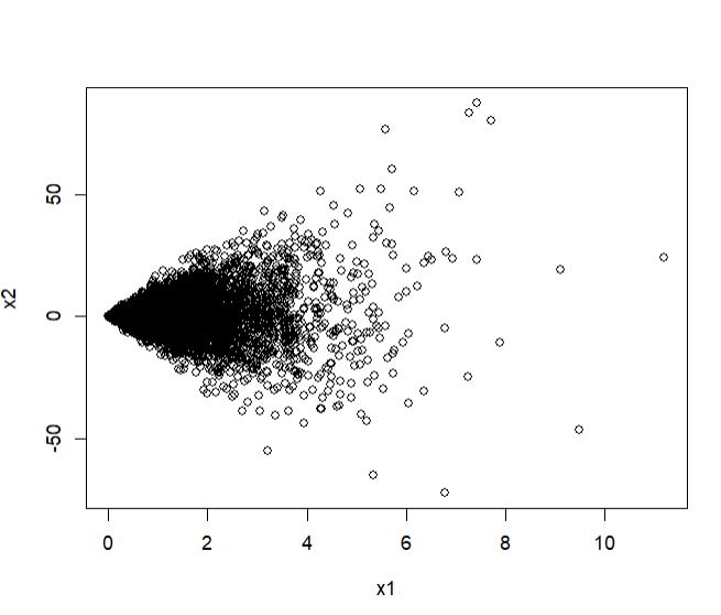
I wrote up a simulated example of the notion I’m getting at. Suppose X1 is a positive-only variable that is not associated with Y, our binary outcome of interest. However, it increases the variance of X2, a variable which does associate with Y. More formally:
- X1 \sim Gamma(\alpha = 1, \theta = 5) (a gamma-distributed variable with a shape parameter of 1 and a scale of 5)
- X2 \sim N(0, \sigma = X1) (a normally-distributed variable with a mean of 0 and a standard deviation equal to X1)
- Y \sim Bernoulli(\pi), a binary variable whose probability of occurrence (\pi) is dependent on X2 but not X1
This makes it so that X2 has a fan-shaped scatterplot with respect to X1 (since X1 determines its standard deviation):
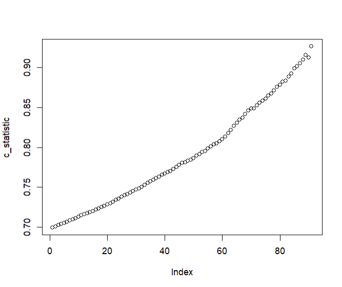
Consequently, when we plot C-statistics of Y (using X2 as the predictor) at increasing cutoffs of X1, we get a plot that looks like so:
In the above example, X1 is useless at predicting Y (the C-statistic will be 0.5 within simulation error); however, it determines the extent to which X2 is able to predict Y.
I’ve attached the code below in case it helps:
#N of patients
n <- 10000

#Set seed
set.seed(100)

#X1; a continuous positive variable with a mean of 5. Not associated with y but scales x2.
x1 <- rgamma(n, shape = 1, scale = 5)

#X2; a variable that scales with x1. Associated with y.
x2 <- rnorm(n, mean = 0, sd = x1)
plot(x1, x2)

#Y; a binary variable that is only determined by x2.
logits <- x2 + rnorm(n, 0, 10)
probs <- plogis(logits)
y <- rbinom(n, 1, prob = probs)

#Calculate C-statistics
library(survival)
#Overall
concordance(y ~ x2)
#When x1 is below its mean
concordance(y[x1 > 1] ~ x2[x1 > 1]) #High C-statistic (x2 varies a lot and is thus able to discriminate well)
#When x1 is above its mean
concordance(y[x1 < 1] ~ x2[x1 < 1]) #Low C-statistic (x2 does not vary a lot and is thus unable to discriminate well)

#Get C-statistics at increasingly greater cutoffs of X1
lapply(quantile(x1, seq(0.05, 0.95, 0.01)),
       function(cutoff)
         concordance(y[x1 > cutoff] ~ x2[x1 > cutoff])$concordance
       ) -> c_statistic

#Unlist and plot
c_statistic <- unlist(c_statistic)
plot(c_statistic)
1 Like
I wasn’t aware that the c-statistic was being used in this way - I would have thought maybe the explained variation in Y given by the variable of interest would be more useful here.
This could be a silly idea, but what if you did it like a LOO-CV; left out each value of the continuous variable and recalculated the AUC? You could maybe find some areas where it overperformed by leaving out some groups.
2 Likes
@Ahmed_Sayed nice work. What I’m lacking is an understanding of the fundamental clinical question you are trying to answer, and why as @robinblythe stated, explained outcome variation or some other measure would not be more relevant. If the outcome were continuous I would have thought the following would be more direct: Compute the residual for each person and run a loess smoother relating age to the absolute residual. This estimates absolute prediction error as a function of age.
2 Likes
For continuous outcomes that approach definitely sounds quite doable and would tackle the question in a straightforward manner.
The clinical question I had in mind was like so: We have a marker X which ranges (for example) from 0 to 1,000. We know there’s a strong linear association between levels of said marker and one’s risk of death.
This association does not vary with age. As such, when one measures X in younger and older individuals, one finds the same HR for low vs high levels of the marker (let’s say a HR 5.0 for comparing values of 100 vs 900 in both younger and older individuals).
However, the problem is that X varies very little for younger individuals. Almost everyone has values that are very close to 0. Therefore, despite the strong linear association that does not vary with age, X offers little clinical value in younger individuals.
For older individuals, there’s a more uniform spread of values from 0 to 1,000. Therefore, X provides some important clinical value.
Calculating the C-statistic in these 2 groups separately would provide us with an important piece of information: X is much better at risk-discrimination among older vs younger adults. This despite effect sizes being identical for both age-groups.
The question thus becomes how do we analyze the data so as to describe the age-dependent discriminative value of X?
One idea that avoids the need for describing the change in the C-statistic I had in mind might be like the following: Calculate the 25th and 75th percentiles of X across the spectrum of age using quantile regression. Then, graph the HRs comparing the age-dependent percentiles of X. This would make it so the HR actually represents comparisons that are realistic for each age (you’d go from an HR of 1.10 at 20 to an HR of 10.0 at 80; not because X interacts with age but rather because the values of X being compared are very different in those aged 20 vs those aged 80).
For continuous variables, I think that’s definitely a viable approach. Thanks for the suggestion! But I’m not sure if it extends to binary variables as well.
I think the LOO might work, but then the question becomes do I leave out one value at a time (I imagine this might be somewhat noisy in smaller datasets)? or do I sort of pick a moving window of values to remove?
At its core my intuition is that it might be similar to the threshold approach I used above where you’re continuously recalculating the C-index by leaving out values above some threshold of X1 (except in this case you’re leaving out particular values of X1 rather than those exceeding some threshold).
1 Like
I think the approach used here for binary Y is exactly what you need. See the graph towards the end where the clinical utility of measuring cholesterol varies strongly with age: 19 Diagnosis – Biostatistics for Biomedical Research
When possible I recommend framing questions on a per-patient basis, not on pairs of patients as the c-index does.
2 Likes
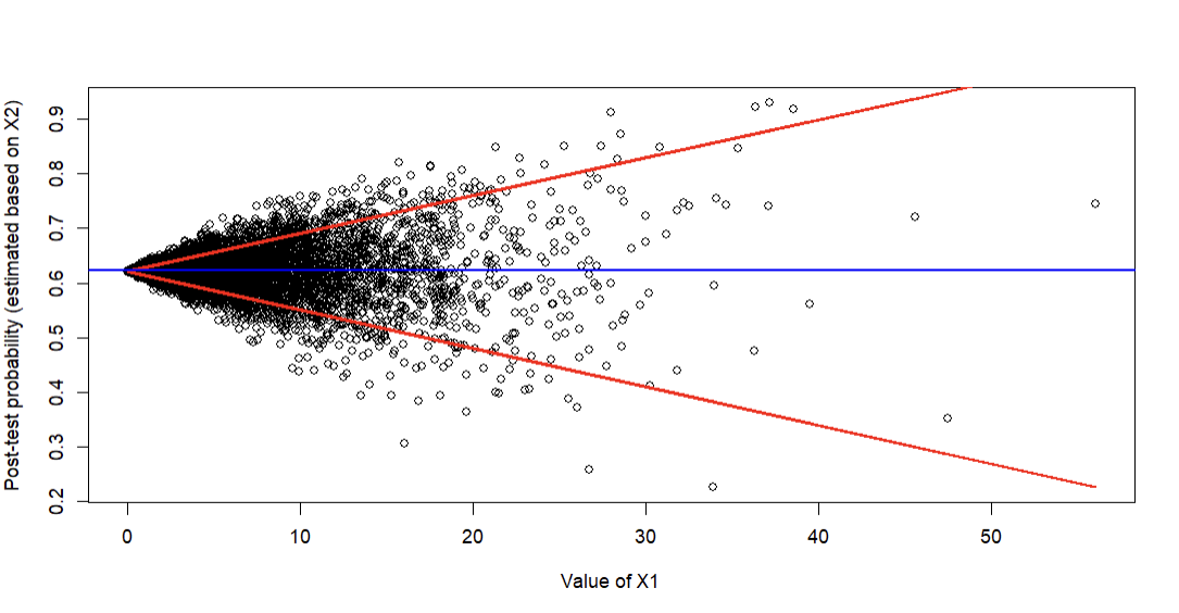
Ahh, thank you for that suggestion! I slightly modified the approach to come up with the following (red lines are estimated 10th and 90th percentiles of predicted probabilities based on quantile regression; blue line is mean prevalence):
It’s easy to appreciate that post-test probability estimated based on X2 (the prognostic marker) varies markedly based on X1 and is really only clinically helpful when X1 is moderate/high (because that’s when predictions start to deviate from the blue line representing the average baseline prevalence). One could also do this using the log-odds instead of probability of course.
To convey uncertainty, I assume one could show the 95% CIs for quantile regression (though I understand those don’t incorporate the original uncertainty in the logistic model’s predictions).
To formally “test” whether there is sufficient evidence that the added predictive value of X2 is dependent on X1, I assume one could report the slope (+ 95% CIs / P-values) for either/both quantile regression lines. Or maybe interquartile differences if the quantile regression uses splines.
1 Like
Wonderful. For an assessment of changes in relative impact (logit scale), formal interaction tests, possibly including nonlinear terms, are called for.
1 Like
In this case, I think an interaction term within the model itself (X1:X2) wouldn’t quite capture the effect since the coefficient of X2 does not depend on X1. Instead, the same coefficient gets multiplied by increasingly larger (negative or positive) values of X2. I think the only way to get at this would be to test the predicted log-odds directly, since the model itself has no notion of the relation between X1 and X2 (that the former increases the variance of the latter).