This study used a propensity score matching (PSM), with a 1:1 nearest-neighbour matching algorithm (with maximum calliper width of 0.01). The balance between covariates after propensity score matching was evaluated through standardized mean differences (SMD). SMD < 0.10 implies adequate balance.
I learned that PSM should not be used. I would like to get the incidence rate after adjustment. How can I do this without using PSM? I was thinking of doing poisson / negative binomial model (using time-to-event data [in years] as an offset variable), but I don’t think that’s possible given I am looking at patient-level data, where patients either developed or did not develop BP. I don’t know if it works with logistic regression, but then, that would give estimates in the odds ratio.
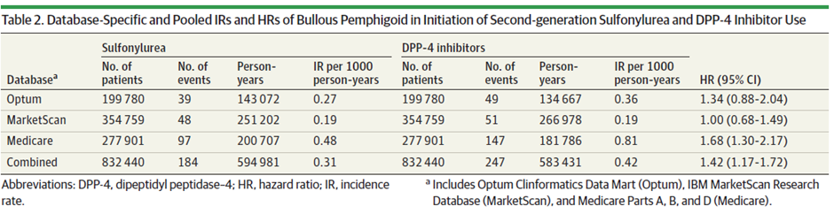
This is the table from the study that I would like to replicate. Would appreciate any advice. Thanks!
Correct, propensity score matching is pretty much a disaster
If you are interested in a single number summary IR per 1000 person-years, making such a simple summary implies a lot of sweeping interesting incidence curve shapes under the rug, so you might as well consider fitting a simple exponential survival model which can easily estimate events per person years
Also, what is the incidence curve method that I can use with the simple exponential survival model? Is this the same as the KM cumulative incidence function?
Let me add to Frank’s answer.
First. I also tend to oppose propensity score matching unless the researcher has a very good justification.
There are three ways off the top of my head to obtain adjusted incidence rates.
Through matching, only not propensity score-based. Frank will hate me for suggesting that, but there is a compelling argument for it, see this answer by Noah on Cross Validated, and I’ll let you be the judge.
Through using propensity scores but with inverse probability weighting instead of matching. Given the IP-weights you could then run a weighted Kaplan-Meier model and use it to obtain the incidence rate. See Cole and Hernan.
You could indeed use Poisson regression (or quasi-Poisson/negative-binomial) to estimate the incidence rate ratio directly after adjusting for other covariates. Poisson regression still works for binary “count” data (they are still counts, they just count once ). Since people with an event are no longer eligible to be further counted, I think you could use the time-of-event as an offset to explicitly set their follow-up time.
I do agree with Frank, though, that if you go through the trouble of repeating the analysis, you would benefit more from plotting the entire cumulative incidence rate curve (the reciprocal of a survival curve) rather than just report one incidence rate scalar.
Without further understanding rationales, I feel that probability weighting, like matching (but not as bad) should be avoided because of inefficiency and difficulty of interpreting final results, and that other models are better fitting than Poisson.
A very valid remark about interpretability, though in the current climate of statistical literacy, that’s the exact reason I once found myself advocating for IPW as a way to prevent colleagues from committing a Table-2 Fallacy
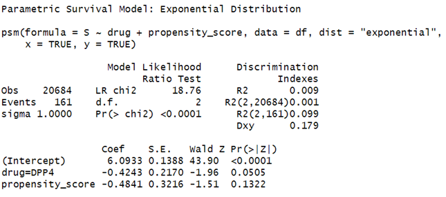
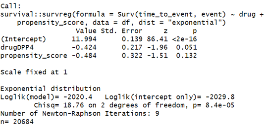
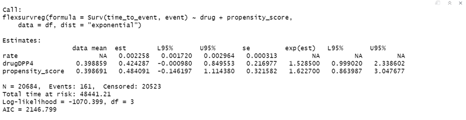
(1) I tried the exponential survival model using rms::psm, survival::survreg and flexsurv::flexsurvreg. The first two produced the same estimates (-0.4243), but the last one gave a different number (0.4243). Do you know why?
(My drug variable is binary with categories DPP4 vs Non-DPP4)
~~
~~
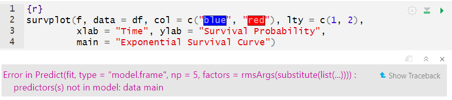
(2) I wanted to plot the psm object (f below) using survplot, but not able to do so. Is it due to the the additional covariate i.e. propensity_score or am I missing some argument?
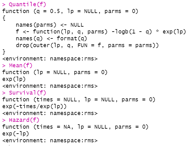
(3) I understand that I can get the adjusted incidence rate (number of event per person-years) from 1/mean of an exponential survival model. Can I get this for individual groups? How do I interpret the results from Quantile.psm, Mean.psm, Survival.psm, and Hazard.psm?
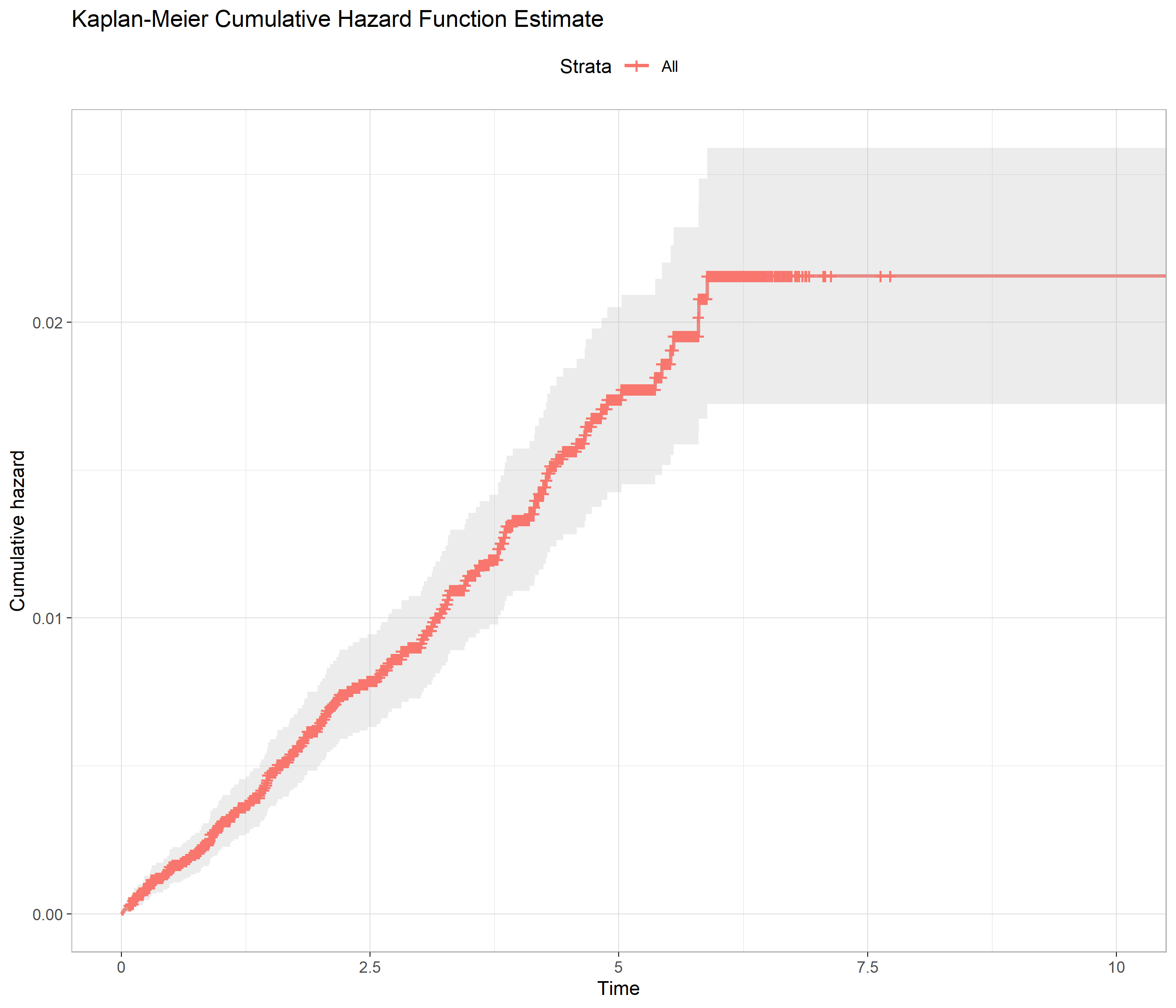
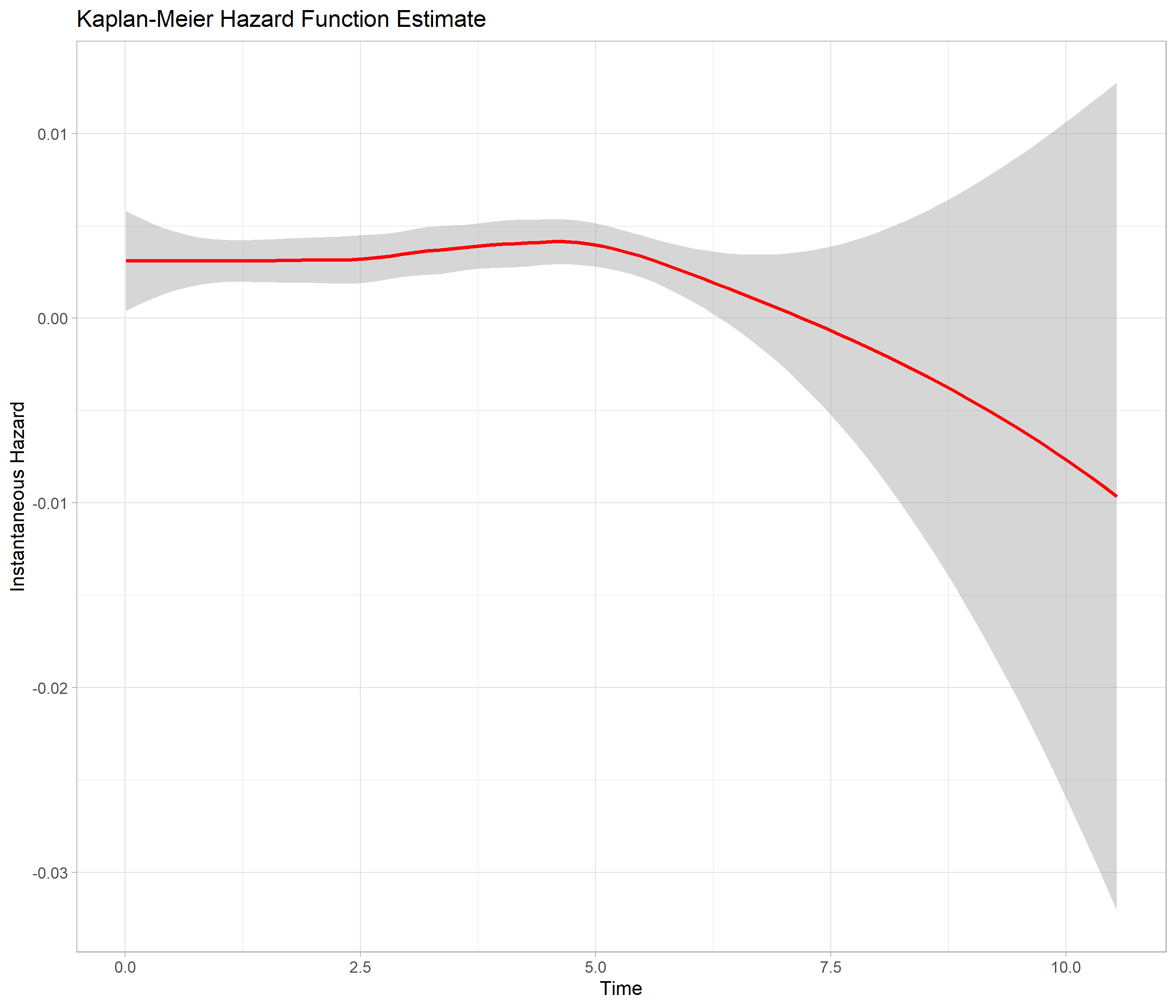
(4) I plotted the Kaplan-Meier cumulative hazard function estimate (using survminer::ggsurvplot) and the KM hazard function estimate (using epiR::epi.insthaz). This is done without any covariates. The hazard does not seem constant. Is it still okay to use exponential?
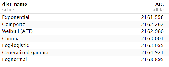
However, I ran various parametric models (“Exponential”, “Weibull (AFT)”, “Gompertz”, “Gamma”, “Lognormal”, “Log-logistic”, “Generalized gamma”) using flexsurv::flexsurvreg and found that exponential has the smallest AIC. Hence, does this mean using exponential dist. is okay?
I don’t think you can compare AIC in different model families.
You know enough to exclude exponential.
Note that if propensity score PS is a probability you need to model it as logit(PS) in the outcome model, and even better spline it to not assume linearity in logit(PS).
Thank you Prof Harrell for responding to my questions.
I have decided to use the cox PH model as I don’t want to make any assumptions about the shape of the hazard function. However, I have a few questions to ensure that my understanding is correct. This is my fit:
f <- cph(S ~ drug + rcs(logit_propensity_score, 5), # 5 knots, 4 df
         data=df, x=TRUE, y=TRUE, surv = TRUE, time.inc=1)
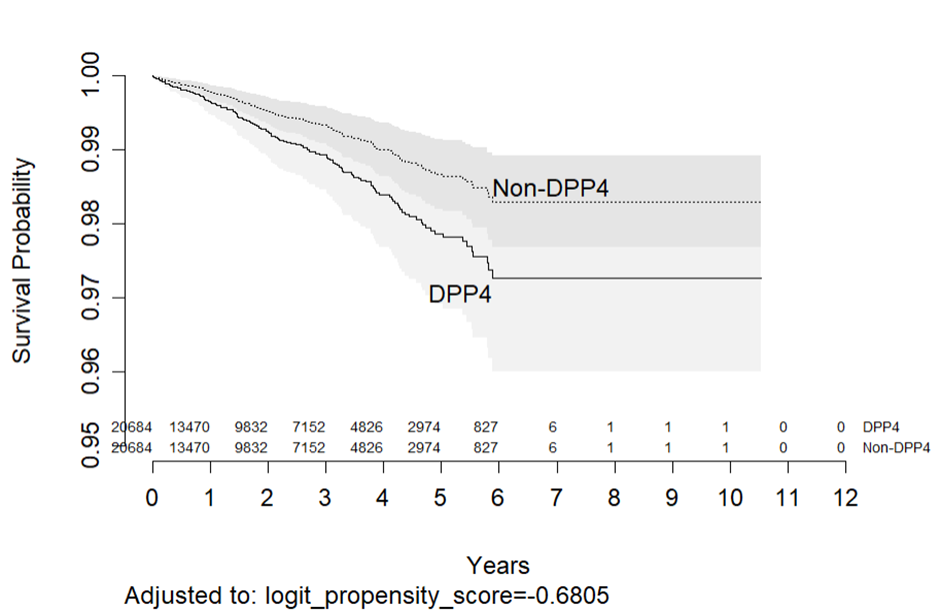
I ran the plot of estimated survival curves. I used the option to print the number of subjects at risk. But instead of giving the numbers for individual groups, I obtained the overall numbers. How do I rectify this? survplot(f, drug, conf.int=.95, n.risk = TRUE, ylim = c(0.95, 1), xlab = "Years")
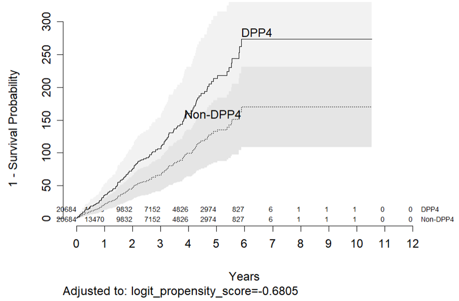
If I consider fun argument as follows, will this give the cumulative incidence per 10,000 per-years? survplot(f, drug, fun=function(y) 10000*(1 - y), conf.int = .95, n.risk = TRUE, xlab = "Years", ylab = "1 - Survival Probability")
When modeling the group variable (assuming PH) all groups are used in estimating all the steps of S(t). To have different numbers at risk requires stratifying on rather than modeling the group variable.