In 2022, Fraiman et al published a controversial paper about the adverse events of COVID vaccines. It was controversial primarily because many felt that it not only has flaws, but that its mistakes are not random, rather, they all point to the direction to show vaccines in a bad light (for instance, it compiled a risk/benefit balance based on data that only had around two months of follow-up – when likely most of the side effects arose, but only a fraction of the benefit); but now I wish to focus on a purely statistical aspect of the paper.
One interesting choice of the analysis was the way it counted serious adverse events (SAEs). Usually the proportion of patients with SAE is calculated as k_{\mathrm{pat}}/N if we have k_{\mathrm{pat}} patients with SAE out of N subjects. k_{\mathrm{pat}}/N is always between 0 and 1, and its complement, 1-k_{\mathrm{pat}}/N is also well-defined and meaningful, i.e., k_{\mathrm{pat}}/N is a true proportion. Instead of that, the authors chose to count not the number of patients with SAE, but rather the number of SAEs. If we have m possible SAE for each patient that implies a proportion of \frac{k_{\mathrm{SAE}}}{mN}, where k_{\mathrm{SAE}} is the number of SAEs. Its a bit more strange metric (meaning something like: the proportion of actual SAEs realized out of all possible ones), but nevertheless, \frac{k_{\mathrm{SAE}}}{mN} is also a valid, true proportion.
Instead of these, the authors however chose a third way to calculate, a hybrid approach combining the above two: they took k_{\mathrm{SAE}}, but still divided it with N. What they got this way, \frac{k_{\mathrm{SAE}}}{N} is no longer a true proportion, but rather a mean event count per participant.
(Sidenote: why the authors chose to count events instead of patients at the first place, even for the SAE part of their analysis, is unclear to me. Perhaps they wished to increase the numbers to have better statistical power. Perhaps they wished to measure some kind of a ‘‘SAE burden’’, but this would be a very strange metric.)
And at this point we arrive to the statistical issue. The crucial problem is that the authors did not have access to individual patient data, only to the aggregates. From these data, it could be seen that the number of SAEs is higher than the number of patients with SAE, i.e., that some patients suffered multiple SAEs, but the authors had no way of knowing who suffered which SAE. That’s not a problem from the point of view of the point estimate (i.e., \frac{k_{\mathrm{SAE}}}{N}), but definitely a problem when estimating its variance. This variance is 1/N^2 times the variance of k_{\mathrm{SAE}} which is the sum of the presence of SAE for each patient and each SAE, and while patients might be assumed to be independent, SAEs are definitely not, so we cannot just sum the variances of each Bernoulli-distributed indicators (which is p\left(1-p\right) simply).
The authors realized this problem, and offered the following solution: “Because we did not have access to individual participant data, to account for the occasional multiple SAEs within single participants, we reduced the effective sample size by multiplying standard errors in the combined SAE analyses by the square root of the ratio of the number of SAEs to the number of patients with an SAE” (p. 5799). They gave no further justification in the paper why this correction is appropriate, how they arrived to it, or any discussion on how good it is, if we consider it to be an approximation.
Some critics, such as Black and Evans, 2023 and Grimes, 2025 criticised the calculation of the standard errors, even after this correction, but similarly gave no further statistical discussion to their position.
So what I found intriguing is that (according to my best knowledge!) none of the involved parties provided any quantitative justification whatsoever for their position. The original authors acknowledged the problem as a limitation, but gave no quantitative investigation on how good their correction is, critics said that it is not acceptable, but also gave no quantitative investigation on how bad the situation is according to their view.
The surprising in that is that I find the problem pretty easily tractable. So either I am wrong that no-one has done it already, or I am wrong that it’s easy statistically, but in either case, I thought it worth posting it ![]()
Here is my take on the issue: I consider the above to be an example of a two-part (hurdle) model. The first part is that we consider patients to be independent; this is true in every abovemention approach, and I’ll also maintain it. This means that each patient is a Bernoulli trial with a parameter of k_{\mathrm{pat}}/N. Once we have the patients with SAE, we model the number of SAEs within them as a zero-truncated distribution. The calculations are straightforward: we can obtain the overall variance using the law of total variance, \mathbb{D}^2\left(Y\right) = \mathbb{E}\left[\mathbb{D}^2\left(Y \mid X\right)\right] + \mathbb{D}^2\left[\mathbb{E}\left(Y \mid X\right)\right], in this case \mathbb{D}^2\left(\widehat{k_{\mathrm{SAE}}}\right) = N \cdot \frac{k_{\mathrm{pat}}}{N} \cdot \sigma^2 + N \cdot \frac{k_{\mathrm{pat}}}{N} \cdot \left(1-\frac{k_{\mathrm{pat}}}{N}\right)\cdot \mu^2 = k_{\mathrm{pat}} \cdot \sigma^2 + k_{\mathrm{pat}} \cdot \left(1-\frac{k_{\mathrm{pat}}}{N}\right)\cdot \mu^2, where \mu and \sigma^2 are the mean and variance of the distribution of the SAE count within affected patients. But we have only one information to estimate this distribution, its mean value, so we will use method of moments, meaning that \mu must be \frac{k_{\mathrm{SAE}}}{k_{\mathrm{pat}}}. Therefore the final result is: \mathbb{D}^2\left(\widehat{k_{\mathrm{SAE}}}\right) = k_{\mathrm{pat}} \sigma^2 + \frac{k_{\mathrm{SAE}}^2}{k_{\mathrm{pat}}}\cdot \left(1-\frac{k_{\mathrm{pat}}}{N}\right) = \frac{k_{\mathrm{SAE}}^2}{k_{\mathrm{pat}}}\left(1 -\frac{k_{\mathrm{pat}}}{N} + \frac{\sigma^2}{\mu^2}\right).
This view is not perfectly universal (as the hurdle nature itself induces some dependence, for example, I think it is not possible to reproduce complete independence in this framework), but seems to be pretty reasonable both statistically and medically. Let’s compare it to the other approaches: the naive estimator’s variance is k_{\mathrm{SAE}} \cdot \left(1-\frac{k_{\mathrm{SAE}}}{N}\right), which is clearly incorrect, while the Fraiman et al corrected estimator’s variance is \frac{k_{\mathrm{SAE}}^2}{k_{\mathrm{pat}}} \cdot \left(1-\frac{k_{\mathrm{SAE}}}{N}\right). This is still incorrect, but now we also see how much: as the difference between 1-\frac{k_{\mathrm{pat}}}{N} and 1-\frac{k_{\mathrm{SAE}}}{N} is miniscule, its error essentially depends only on \sigma^2 (and the number of affected patients). Thus we learned that Fraiman et al is correct – at least under the hurdle model – if and only if \sigma^2=0, i.e., if every affected patient suffers exactly the same number of SAEs (which is not only extremely unlikely, but physically impossible if \frac{k_{\mathrm{SAE}}}{k_{\mathrm{pat}}} is not an integer) and that their corrected variance is always an underestimation of the true variance.
This is already an important finding in my view. The last question is: What is the bias, how wrong this approximation is? To answer this, we need to address the only remaining open issue in this framework: the choice of the appropriate distribution for the SAE count within affected patients.
A logical first choice is zero-truncated Poisson (ZTP). ZTP with a parameter of \lambda has a mean of \frac{\lambda}{1-e^{-\lambda}}, so we have to solve the \frac{\hat{\lambda}}{1-e^{-\hat{\lambda}}} = \frac{k_{\mathrm{SAE}}}{\mathrm{pat}} equation. Unfortunately this equation does not admit a closed-form solution, but is pretty easy to solve numerically, or, in this particular case, we can simply use the Lambert W function.
To immediately show a concrete illustration, I’ll use data from the treated group of the Pfizer trial, which had 103 patients experiencing 127 SAEs out of the 18,801 subjects. (This includes only those who were followed for at least 1 month after Dose 2; this was used by the Fraiman et al paper, so I used this as well for consistency.) Here is the code:
kPatient <- 103
kSAE <- 127
N <- 18801

lambdaZTP <- kSAE/kPatient + lamW::lambertW0(-kSAE/kPatient * exp(-kSAE/kPatient))

kSAE * (1 - kSAE/N) # Naive estimator
kSAE^2/kPatient * (1 - kSAE/N) # Fraiman et al corrected estimator
kPatient * ((lambdaZTP+lambdaZTP^2)/(1-exp(-lambdaZTP)) -
              lambdaZTP^2/(1-exp(-lambdaZTP))^2) +
  kSAE^2/kPatient * (1 - kPatient/N) # ZTP
That is, we have the following results:
| Method | Variance | Standard error |
|---|---|---|
| Naive estimator | 126.1 | 11.23 |
| Fraiman et al corrected estimator | 155.5 | 12.47 |
| True value under ZTP | 181.3 | 13.47 |
So, Fraiman et al indeed increased the standard error estimate by about 10% as they claimed (p. 5799) – but it is simply not enough! Assuming the ZTP model, the correct factor should have been 19.9%, twice what they have used.
At this point, it perhaps worth mentioning that the smallest variance that we can create with these parameters is of course a distribution that can only take the values of 1 and 2 – this will have the smallest \sigma^2. As we know the mean, the only possibility is p_1 = 0.767 and p_2 = 0.233 (obtained by solving the equation p_1 + 2\left(1-p_1\right) = 127/103) which has a variance of 0.767\cdot\left(1-127/103\right)^2 + 0.233\cdot\left(2-127/103\right)^2 = 0.179. Thus, the variance of k_{\mathrm{SAE}} will be 174.1. That’s barely less then the one in the ZTP model, and still means that an increase of 17.5% would have been needed in the standard error (instead of the 10% they have used). That’s the smallest possible value.
Unsurprisingly then, the distribution of the ZTP with the above \lambda is not really far from this: it takes 1 with a probability of 79.8%, 2 with a probability of 17.4%, 3 with a probability of 2.5 and 4 with a probability of 0.3% (every other probability is below 0.05%); see r actuar::dztpois(1:10, lambdaZTP).
We can run a quick simulation to verify the above results:
simPat <- rbinom(1e6, N, kPatient / N)
total_patients <- sum(simPat)
all_SAEs <- actuar::rztpois(total_patients, lambdaZTP)
iteration_ids <- rep(1:1e6, times = simPat)
simSAE <- tapply(all_SAEs, iteration_ids, sum)
simSAE_full <- numeric(1e6)
simSAE_full[as.numeric(names(simSAE))] <- simSAE

mean(simPat)
var(simPat)
mean(simSAE_full)
var(simSAE_full)
This confirms the above theoretical derivations.
The role of \sigma^2 with a fixed expected value simply means: how heavy the tail is (i.e., how clustered the SAEs are). Luckily we can experiment with this, improving the generality of our results by using zero-truncated negative binomial (ZTNB) instead of ZTP. ZTNB includes ZTP as a special case, so it is indeed a generalization, but is allows us to vary how heavy the tail of the SAE number distribution is – essentially, to vary the correlation structure of the SAEs within an affected patient.
We will have one free parameter to vary (ZTNB has two parameters, but we eliminate one by the constraint on the mean). Perhaps its better to parametrize the problem using mean and dispersion:
library(ggplot2)
theme_set(theme_bw())

getZTNBmu <- function(theta, mean_zt) {
  f <- function(log_mu) exp(log_mu) /
    (-expm1(theta * (log(theta) - log(theta + exp(log_mu))))) - mean_zt
  exp(uniroot(f, interval = log(c(1e-12, mean_zt)), tol = 1e-5)$root)
}

thetas <- 10^seq(-3, 2, length.out = 1000)
res <- do.call(rbind, lapply(thetas, function(theta) {
  mu_nb <- getZTNBmu(theta, kSAE/kPatient)
  var_ztnb <- (mu_nb + (mu_nb^2 / theta) + mu_nb^2) /
    (-expm1(theta * log(theta/(theta + mu_nb)))) - (kSAE/kPatient)^2
  data.frame(theta = theta, kSAEVariance = (kPatient * var_ztnb) +
               kSAE^2/kPatient * (1 - kPatient/N))
}))

probGreaterThan3 <- function(thetas) {
  sapply(thetas, function(theta) {
    mu_nb <- getZTNBmu(theta, kSAE/kPatient)
    (1 - ((pnbinom(3, size=theta, mu=mu_nb) - dnbinom(0, size=theta, mu=mu_nb)) /
            (1 - dnbinom(0, size=theta, mu=mu_nb)))) * 100
  })
}

ggplot(res, aes(x = theta, y = kSAEVariance)) + geom_line() +
  scale_x_log10(breaks = 10^(-5:5), labels = scales::label_log(),
                sec.axis = sec_axis(
                  transform = probGreaterThan3,
                  name = "Probability of having more than 3 SAE [%]")) +
  annotation_logticks(sides = "b") +
  labs(x = "Dispersion parameter", y = "True variance")
The result (in addition to the dispersion parameter, the probability of a patient with SAE having more than 3 SAE is indicated; that is likely a more meaningful and interpretable way to describe dispersion):
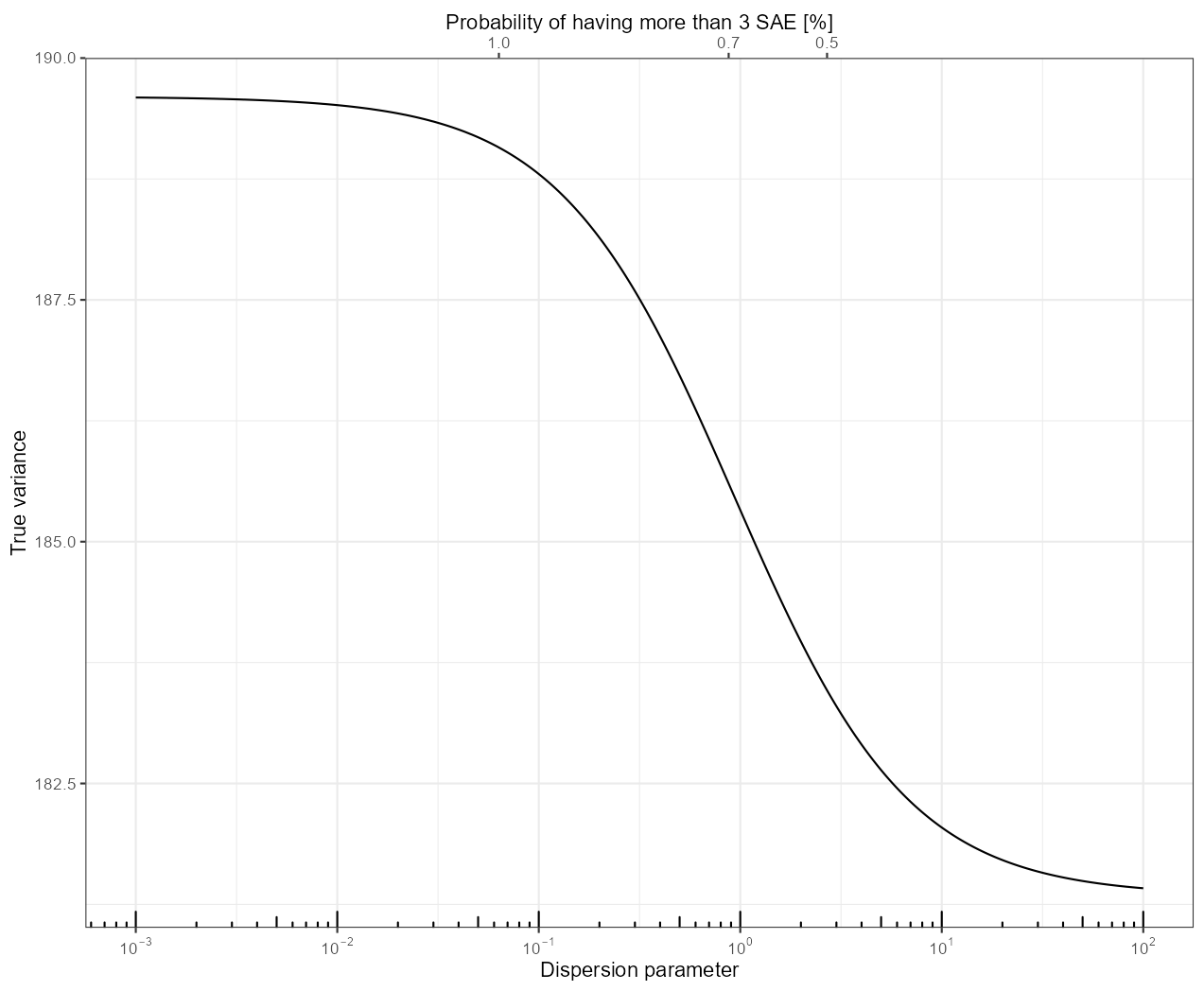
As we can see, the true variance is monotonically increasing as we increase the dispersion.
The takeway is that the ZTP is actually a lucky scenario in terms of how good the correction is: if the dispersion is larger, then – as we have already seen due to the dependence on \sigma^2, but now in a more quantitative way – things get even worse. This is, however, not a large increase compared to what we have already seen with ZTP, with 182.2 going up to around 190 (for a \theta = 0.01, which means around 1% probability to have more than 3 SAEs for an affected patient). This means an increase in the standard error of 22.7%, instead of the 10% used by Fraiman et al.
(It is beside the point, and in some sense it rather just illustrates the problems with frequentist inference, but let me mention that in the SAE part of Table 2 of Freiman et al, the only row where they obtained a significant result was that of the Pfizer trial; neither the Moderna trial nor the combined analysis produced significant result (CI included zero). Fraiman et al considered this sole significance important, as they had a separate section discussing it, beginning with the following paragraph: “In their review of SAEs supporting the authorization of the Pfizer and Moderna vaccines, the FDA concluded that SAEs were, for Pfizer, “balanced between treatment groups,” [15] and for Moderna, were “without meaningful imbalances between study arms.” [16] In contrast to the FDA analysis, we found an excess risk of SAEs in the Pfizer trial. Our analysis of Moderna was compatible with FDA’s analysis, finding no meaningful SAE imbalance between groups.” (p. 5800). Although the authors carefully avoided the word “significant”, it is quite clear that this is what they refer to when saying “we found an excess risk”, as the difference between the Pfizer trial (where they say they “found and excess risk”) and the Moderna trial (where they say they found “no meaningful imbalance”) is that in case of the Pfizer trial their results are significant, but not for the Moderna trial. Now the problem is that this significance is obtained when the naive standard error of 7.87 is increased by about 10% according to their correction, but if we use the ZTP-based correction – of course, here we have to apply it to both arms – which is, as we have already seen, probably conservative, the CI is (-0.0262 to 36.1), i.e., the significance disappears, even for the Pfizer trial.)
So, these are my ideas at first glance of the problem; but I really appreciate any comment, criticism or feedback about these calculations!