I am trying to develop an ordinal model, according to the recommendations of the book Regression Modelling Strategies (Chapter 15).
The aim is to predict quality of life (EORTC ordinal scale, with range 0-100) after breast cancer surgery. In particular, it would be relevant to identify women with good results, e.g., P(QoL>75%) .
I have 217 observations.
I have built a model using some key variables, and I want to test the assumptions of several possible models.
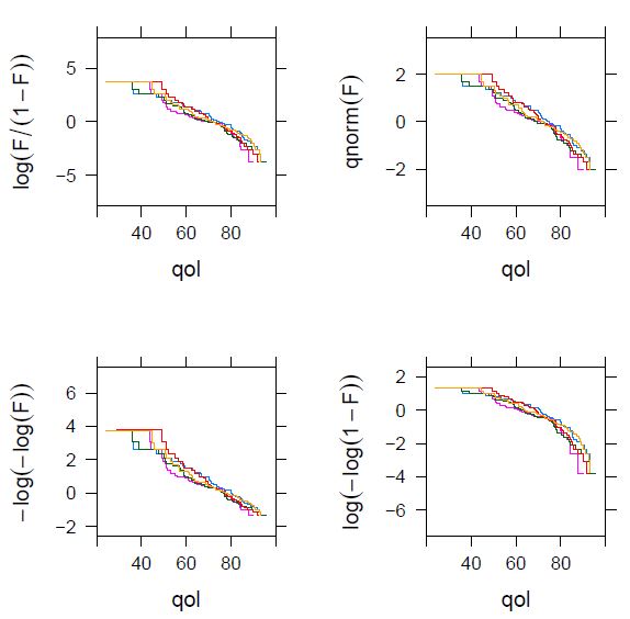
I have obtained this plot, which is nowhere near as beautiful as the one in the book:
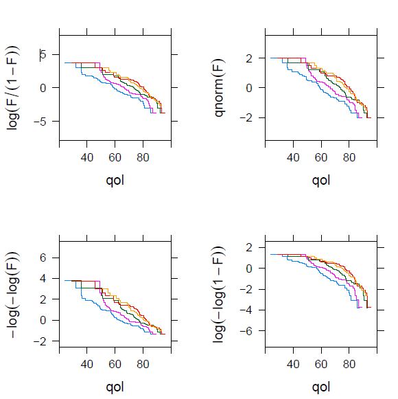
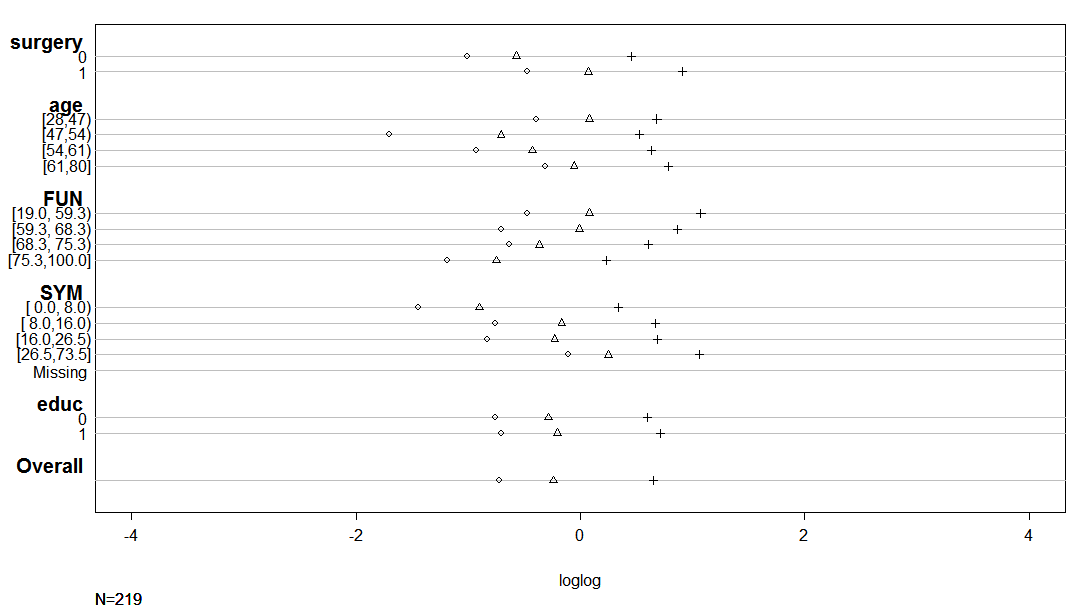
I have doubts about whether the log-log link is still reasonable here. On the other hand, the output shows the slopes for several models. I don’t know how to get the slopes for the loglog link (instead of the cloglog). I think it could be useful to expand here the explanation of how these plots are interpreted.
This is the code:
f <- ols (qol ~ surgery +rcs(age,3) + pol(EORTC), data=qol)
qolf <- fitted (f)

p <- function (fun , row , col ) {
  f <- substitute (fun ); g <- function (F) eval(f)
  z <- Ecdf( ~ qol , groups =cut2(qolf , g=5),
             fun=function (F) g(1 - F),
             ylab=as.expression(f), xlim=c(20, 100),  data=qol,
             label.curve =FALSE)
  print (z, split =c(col , row , 2, 2), more=row < 2 | col < 2)
}
p(log(F/(1-F)), 1, 1)
p(qnorm (F), 1, 2)
p(-log(-log(F)), 2, 1)
p(log (-log(1-F)), 2, 2)
# Get slopes of pgh for some cutoffs of Y
# Use glm complementary log-log link on Prob(Y < cutoff) to
# get log-log link on Prob(Y ??? cutoff)
r <- NULL
for (link in c( "logit" , "probit", "cloglog"))
  for(k in c(40,50,60,70,80,90)) {
    co <- coef(glm (qol<k ~ qolf , data=qol, family =binomial (link)))

    r <- rbind (r, data.frame (link=link , cutoff =k,
                               slope=round(co[2] ,2)))
  }
print (r, row.names =FALSE ) #
… and the slopes:
> print (r, row.names =FALSE ) #
link cutoff slope
logit 40 -0.15
logit 50 -0.13
logit 60 -0.13
logit 70 -0.15
logit 80 -0.13
logit 90 -0.18
probit 40 -0.08
probit 50 -0.08
probit 60 -0.08
probit 70 -0.09
probit 80 -0.08
probit 90 -0.09
cloglog 40 -0.13
cloglog 50 -0.11
cloglog 60 -0.10
cloglog 70 -0.10
cloglog 80 -0.07
cloglog 90 -0.07