Dear fellows,
I am dealing with a Cox PH model with n = 666 observations and 501 events. Covariates (26, 10 categorical and 16 continous)
Basically, I performed this steps:
- Basic data statistics, dataset cleansing
- Categorisation of covariates
- Log-rank test and Kaplan-Meyer plots
- Full-model linear
- Somers’ Dxy rank correlation between predictors, variable clustering and redun() analysis
- Removed and modified some covariates from domain knowledge
- Full-model with splines (4knots)
- Reduction d.f. of splines (starting from those less important covariates, taken from their relative explained likelihood)
- Pooled test of interactions, added those that improve AIC in X2 scale and do not affect rough shrinkage keeping it >0.9.
The best model I have developed, is the following:
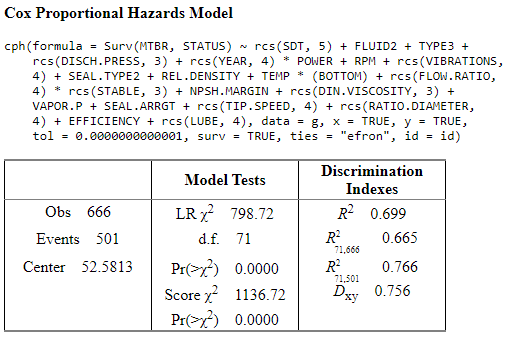
n= 666
Concordance= 0.878 se= 0.006487
concordant discordant tied.x tied.y tied.xy
166303 23099 2 18396 0
extractAIC(model)
[1] 71.000 5316.372
AIC in X2 scale: 656.7211
Rough shrinkage = 0.9111079
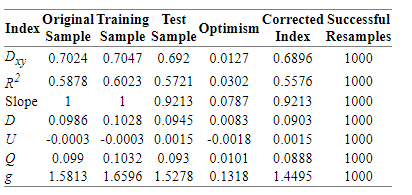
The result of validate() function with method=“boot”, maxiter= 2000, B = 1000 is:
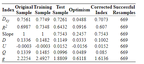
As far as I know this model would have shrinkage with new data, so I may follow further steps in order to improve its performance.
As well, I would need some insights in interpreting these bootstrapping results.
Could anyone give me some give of the following steps to follow?
I assume that some more data reduction would be necessary, but I would like to have an idea of which way would be better.
Note: I need to have interpretability of the effect of the covariates, so I do not feel confortable in using a PC methodology for reducing the dimensions.
Thank you in advance for your help!
It appears that the rough heuristic shrinkage estimate is too rough for this example, as compared to the bootstrap. 71 parameters is a lot. I think you need to go back to subject matter thinking. Note that if testing groups of interaction terms you need to remove them all or keep them all. Doing variable selection on individual terms is not recommended.
Thank you Frank for your quick reply.
All of this applies to a Cox PH model.
It appears that the rough heuristic shrinkage estimate is too rough for this example, as compared to the bootstrap. 71 parameters is a lot.
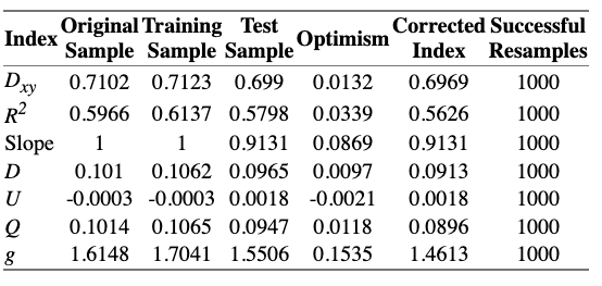
I am reagrouping similar categories of two intensive covariates (those that introduce many d.f. to the model) and I have reduced 10 d.f. of the total model. I still have 62 d.f., but most of them come from the splines approaches wich, by the way, increase satisfactorily the LR R2 of the model.
Could be a good rule of thumb to continue working on it until having an slope optimism < 0.05?
I understand that this is a matter of overfitting vs LR R2 maximisation…
I think you need to go back to subject matter thinking.
I do not know exactly what do you mean, maybe you refer to reduce the number of covariates from the beginning of the model developing?
Note that if testing groups of interaction terms you need to remove them all or keep them all. Doing variable selection on individual terms is not recommended.
What I did is:
- Make 4 groups of covariates taht contain only those variables which from my expert knowledge have sense to interact with each other.
- Ran 1 model for each group, each model contain all the possible interactions. (x1+x2+…)^2
- Ran fastbw() for each model and took only those interactions that remain in the final model given by fastbw() function with aic criteria.
- Include each “important” interaction (detected in 3.) one-by-one in the full-model and check if it improves AIC and likelihood. If not, I do not use it and if yes I add to the final model.
Doing this approach I get 4 interactions that contribute to the final model, which in fact have very good sense.
Honestly, I do not know if it is statistically correct or not, that’s why I would like to go a little deeper in this topic and see if it’s sufficiently robust and acceptable.
Regards,
Marc
Try the “pre-specify complexity” strategy at the start of Chapter 4 of RMS.
1 Like
Dear professor,
i’ve been reading and testing how to manage the interaction effects in my model and I continue struggling with it. I would be very grateful if some additional light comes from this forum.
Note that if testing groups of interaction terms you need to remove them all or keep them all. Doing variable selection on individual terms is not recommended.
My questions are:
1.- I understand that the method of pooling interaction effects need to check the significance of the whole group so, depending on the result of the test we should keep or remove all the tested interactions as a whole. Could you please confirm if I am right?
2.- Is it possible to check individually which interactions may be added to the model and which may not? Could the fastbw() help in this?
3.- If it’s not possible, or not robust enough, is because the same reason as we can’t do it with simple covariates when we manage multiple d.f. in our model?
4.- What do you think about including few possible interactions (1 to 10) that are assessed by domain knowledge and penalize the full-model later? would it have statistical sense and supported?
5.- In topic 4.12.1 Developing Predictive Models of Regression Modeling Strategies – 4 Multivariable Modeling Strategies (hbiostat.org) it can be seen that the step 6. Data reduction if needed is performed before step 10. Check additivity assumptions by testing pre-specified interaction terms. My idea was to add interactions before performing a data reduction like (PCA or penalized regression) in order to verify all the possible interactions before reducing the d.f. in order to keep in model as much information as possible before reducing the d.f. In this matter, what is your reccommendations with regards the moment when the interactions may be included in the model?
As always, thank you so much for your help and kind replies,
Yes. But the only really logical strategy is to pre-specify Bayesian priors on all the interaction effects. That incorporates uncertainties and treats interactions as “half in, half out” of the model.
Bad ideas
Yes, plus the fact that interactions are collinear with other interactions and with main effects.
Pretty reasonable. A quick form of Bayes.
- In this context data reduction could be aimed at collinearities among interaction terms by reduction all interaction terms to a few PCs that approximate the whole system of interactions.
2 Likes
Hi,
I tried to work with PCA and I fitted the model with the best comprmise between AIC and number of components (I transformed the original variables with canonical transformation with transcan()).
The optimism of the model with PCA transformed components is much better than what I got before with other models with raw variables, but is still > 0.05…
What are your thoughts about these results? do you think that are reasonable good to go ahead with it and continue the modeling steps?
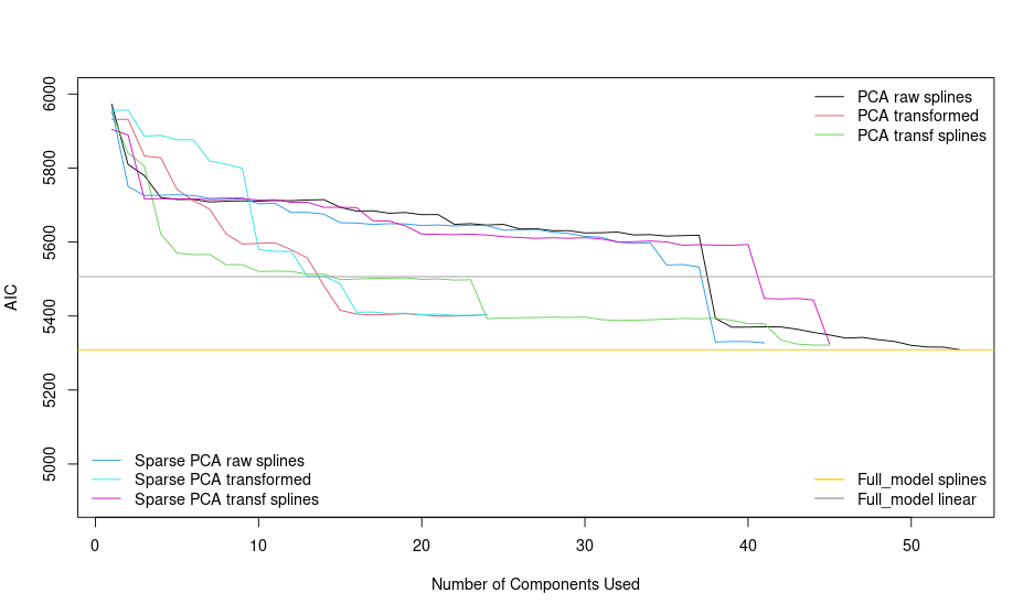
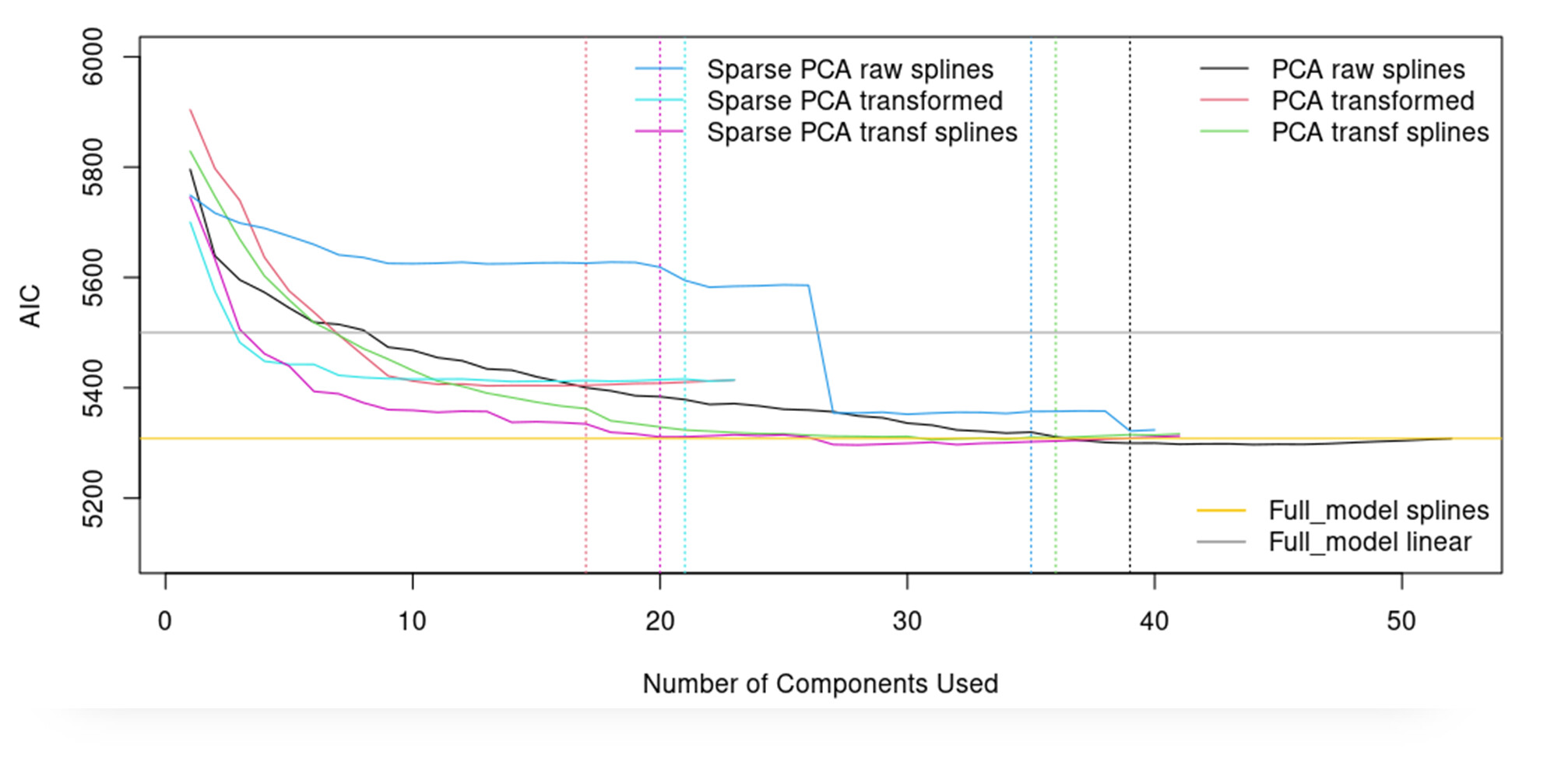
Note: I tried as well sparse principal components analysis but the AIC that I get are significantly higher. (5800 vs 5400)
Thank you so much in advance for your help,
Marc
I’m surprised that sparse PCA did worse but see a lot of promise in your PCA approach.
1 Like
Hi professor, thank you so much for your comments.
Sorry for the confusion…You were correctly surprised about the results of sparse PCA with transformed variables (red), the behaviour is similar or slightly better than the PCA transf var (blue) in terms of AIC. Here you can see the plot:
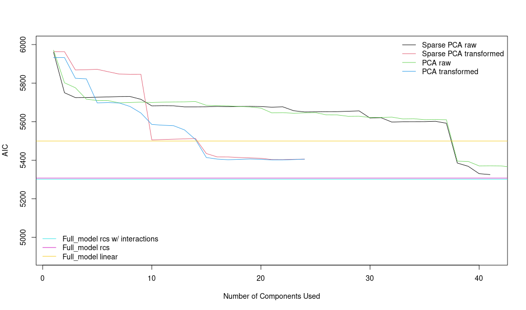
Once this is done, I have now to keep working with one of both.
PCA with transformed variables
Sparse PCA with transformed variables
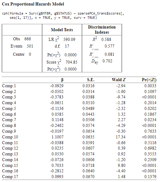
I think that PCA performs better than Sparse PCA, and it has more ‘significant’ components as well and I think that could be better option than Sparse PCA model.
Any thoughts having this additional infomation in hads?
Thank you!
No other thought except make the partial effects plots for the raw-variable models. You may have some extreme, important nonlinearity that was missed by PCA methods.
1 Like
Hi,
I understand that you pointed out the nonlinearity because of the difference between the AIC of full_raw model linear and full_raw model splined. Am I right?
In fact, I did not use exactly the raw covariates for both raw PCA’s (sparse and non-sparse),
prin.raw <- princmp(~ rcs(SDT,5) + rcs(YEAR,3) + TYPE3 + FLUID2 + DOUBLE.SUCTION + TEMP + DISCH.PRESS+ rcs(RPM,3) + POWER + rcs(VIBRATIONS,4) + SEAL.ARRGT + SEAL.TYPE2 + BOTTOM + rcs(FLOW.RATIO,3) + NPSH.MARGIN + REL.DENSITY + rcs(DIN.VISCOSITY,3) + VAPOR.P +rcs(TIP.SPEED,4) + rcs(RATIO.DIAMETER,4) + EFFICIENCY + rcs(Ns,5) + STABLE + rcs(LUBE,3),k=53, sw=TRUE, data=g)
I understand that if the PCA’s are performed from splined covariates, then the Prin.Comp and the cph models later will have this ‘nonlinearity’ embedded in them.
As well, I checked that transcan() transforms the continous variables into restricted cubic splines, so I assumed that the non_linearity has been taken into account in this case as well.
transcan and transace try to pre-transform variables to make them maximally consistent with each other. This is masked to outcomes. It may be that the unsupervised pre-transformation process badly approximated the outcome-based transformations.
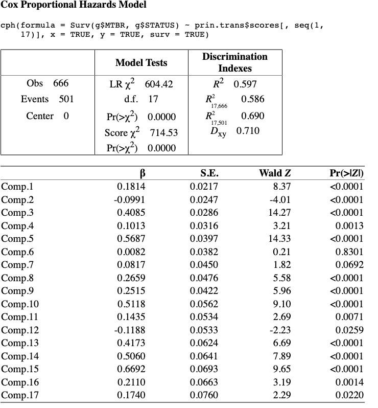
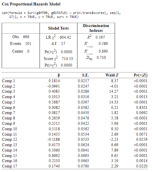
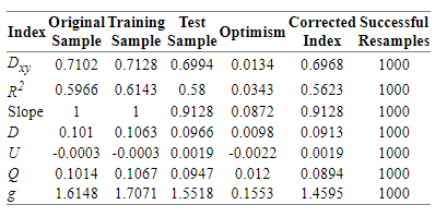
Hi, I made some improvements in the strategy and I transformed again the transcan() variables into splines against the outcome to grasp the unlinearities. The performance of the models with that variables improved and in the limit (max number of components) aproximate to the best achievable AIC by the most complex models.
As the variables are ordered by princmp() and pcapp() by the variance explained I have taken the covariates and reordered by the best ‘performance’ by using BeSS package and looking for the golden section of each model.
See the following: https://www.jstatsoft.org/article/view/v094i04
The d.f. are reduced considerably by taking only the most relevant components, not in order of the dataset until the best AIC is reached, but the most relevant ones.
The model now is:
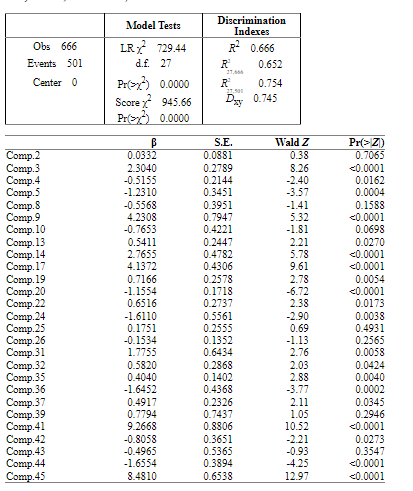
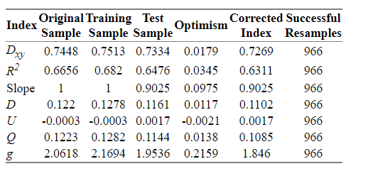
I think that the method looks good, but if there is anything remarkable I would be very grateful to hear from you.
Thanks
Pretty cool. But I worry when the order of selection of PCs is not pre-specified. I see that you have a high signal:noise ratio (R^2) which does make it easier to model.
1 Like
Thank you so much for your valuable comments dr Harrell.
At this time, I have a new question with regards the checking of model assumptions.
I have ‘splined’ vs the outcome all the raw continous covariates before performing the PCA (both standard or sparse) in order to grasp the nonlinearities when fitting the cox model. This can be seen in the plot above.
I’ve done this procedure because if I spline the principal components (once the PCA/SparsePCA is already done) then the degrees of freedom of the model increase again and so the shrinkage and optimism.
The problem that I face now I that the model assumption of linearity seems to be not preserved for some principal components (see the following)
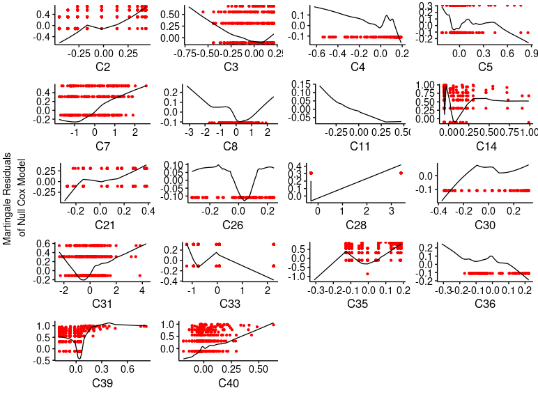
Do you have any explanation of this? Is there a better way to avoid/relax non-linearities restrictions when dealing with principal components?
As well, I found problems with the proportional hazards assessment that I did not have with the raw covariates. Is this phenomena habitual when developing models with PC’s?
Thank you
RMS has examples of nonlinear PCA using the transcan function in the Hmisc package, e.g. this and an earlier chapter. And don’t mess with nonlinearities on PCs after computing them. That’s too late.
As always, thank you for your kind replies dr. Harrell. I have reformulated this post/questions because I feel they were incorrectly focused.
1.- Once a cox model is fitted with restricted cubic splines(adjusting them with anova analysis of nonlinearities and plots of each log-hazard ratio vs covariate), is it necessary to check the linearity cox assumption by checking e.g. martingale residuals?
As these residuals are calculated vs raw covariates, they will not show linear in the plots… am I right?
2.- I can’t find in RMS how to deal with no-linearity with log-hazard ratios with principal components or with transformed variables (e.g. transcan). Maybe I am lost, but honestly I have not found it, I am sorry.
3.- So, what I have done is the following:
I created databases which content is not the raw variables but the splined variables (gathered with non-linearities anova analysis done before).
Later, I transform these (new) splined variables (using e.g. transcan()) and later I perform the PCA.
4.- The problem now is that after fitting the model with the principal components, even though they have been computed from the covariates expanded in splines-basis, the martingale residuals of the cox model do not show linearity.
A concern, and a possible explanation is that the principal components include some categorical variables that have been converted into dummy variables (by princmp()) and maybe they are changing the ‘linearity’ achieved with the splines.
I am little bit struggled with this, maybe I have concept/basis errors, so any help will be very helpful to guide my research in the right way.
Regards,