Hello,
I’m hoping for some advice please @VickersBiostats
Does it make sense to carry out a decision curve analysis for a decision tree model?
Below is an example I have taken from a worked example using the ‘ctree’ function in R (R - Decision Tree) to determine from a set of reading skills whether a person is a native speaker or not. The response variable is binary ‘native speaker’ yes or no and the model outcome is in the same format (i.e. binary yes / no). It is possible from these two variables to calculate the true positive and false positive achieved when using the decision tree.
I have added on some code to create a decision curve. Since there is only one true positive and one false positive (as oppose to with a continuous model outcome / predicted probability where these would vary depending on cut-points) the only thing that changes when calculating the net benefit across the thresholds of the decision curve, is the weighting applied to the false positives. I’m also unsure of how the model outcome would relate to the decision curve thresholds.
Any advice would be appreciated.
Many thanks
Michelle
library(tidyverse)
library(party)
library(caret)
library(dcurves)

# Print some records from data set readingSkills.
print(head(readingSkills))

# Create the input data frame.
input.dat <- readingSkills[c(1:105),]

# Give the chart file a name.
png(file = "decision_tree.png")

# Create the tree.
output.tree <- ctree(nativeSpeaker ~ age + shoeSize + score, data = input.dat)

# Plot the tree.
plot(output.tree)

# Predictions from tree
input.dat$pred <- predict(output.tree)

# Confusion matrix
cm <- confusionMatrix(input.dat$pred, input.dat$nativeSpeaker, positive = "yes")
cm$table

# creat dca object
input.dat$pred <- recode(input.dat$pred, "no" = 0, "yes" = 1)
dca_object <- dca(nativeSpeaker ~ pred, data = input.dat)
plot(dca_object)

# Extract data from dca object
dca_object_df <- dca_object$dca
summary(dca_object_df[dca_object_df $label=="pred",])
You have two options here. From your decision tree, you can either give a probability of 1 for “positive” individuals and 0 for “negatives” or give a probability based on observed probabilities (e.g. if there are 50 individuals at a given terminal node on your tree, and 16 of them have the event, that is a probability of 32%). Now you have a probability and an outcome for every individual and can now run your decision curve.
1 Like
If, on the other hand, this is a question about interpretation, show a picture of your curve along with an explanation of the decision you are trying to make and a rationale for the thresholds shown.
@VickersBiostats thanks so much for the response. My question was a mix of should I use dca in this scenario (which you’ve answered thank you!) and how to interpret.
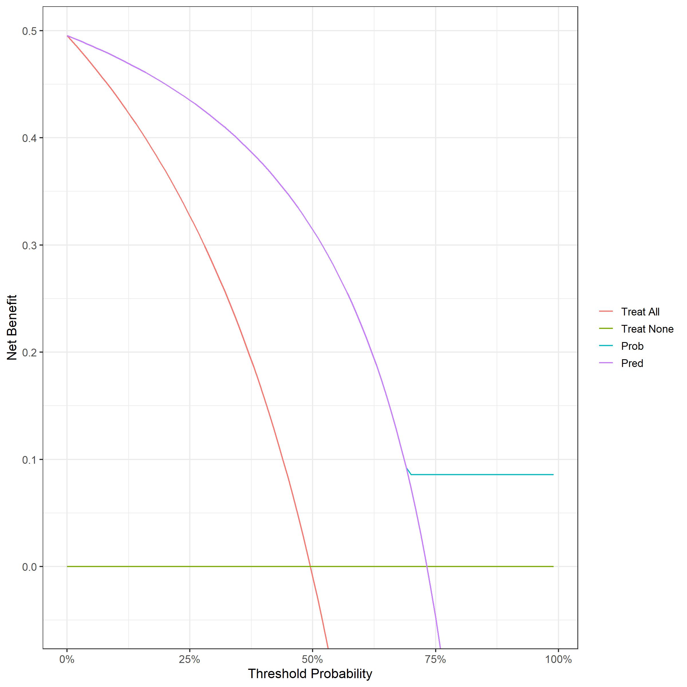
In the code included in my original post, I used 0 or 1 as the probability to feed into the decision curve to give the curve ‘Pred’:
I’m struggling with the interpretation because the outcome is always 0 or 1, so regardless of where your decision threshold is, the 0’s will always be below and the 1’s will always be above.
If I assign probabilities based on observations:
input.dat$node <- attributes(output.tree)$where
xtabs(~ input.dat$node + input.dat$nativeSpeaker)

#                 input.dat$nativeSpeaker
# input.dat$node  no yes
#               4 13   0
#               5  0   9
#               6 21   0
#               7 19  43

# probability for node 4 = 0 (0/13)
# probability for node 5 = 1 (9/9)
# probability for node 6 = 0 (0/21)
# probability for node 7 = 0.69 (43/62)

# Extract probabilities directly
x <- unlist(predict(output.tree, type = "prob"))
index <- 1:length(x)
input.dat$prob <- x[index[index %% 2 == 0]]

dca_object_prob <- dca(nativeSpeaker ~ prob, data = input.dat)
plot(dca_object_prob)
The curve for the model (above shown as Prob) plateaus at 69% (i.e. the only non-0/1 probability) since there are no false positives after this point.
I worry that depending on whether you use the binary 0/1 outcome or observed probabilities leads to different outcomes for some, in this case node 7.
Thanks again for your help!
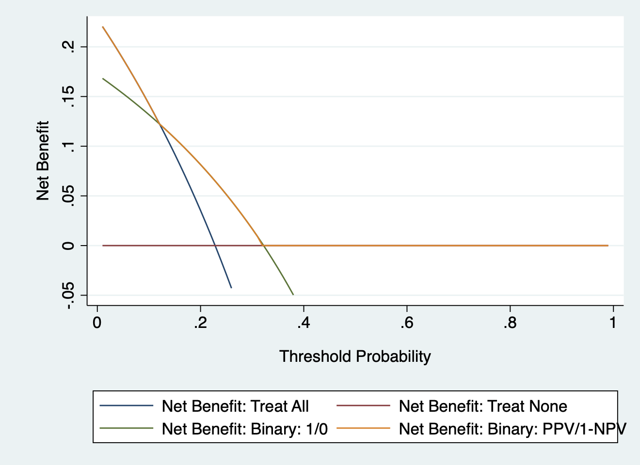
The purple line is exactly what a decision curve for a binary test should look like. You are sort of right that you don’t apply a threshold in clinical practice, but that is the point of binary tests, they are just a 1 or a 0. It is “your test came back positive Mr. Jones, so we will have to give you the treatment” rather than “Mr. Jones, the model has given you a probability of x%. Let’s discuss what to do next”. The blue line is wrong, by the way. If instead of giving probability of 1 and 0 to positive and negative tests, you give probabilities of the PPV and 1-PPV, then the decision curve follows the “treat all” line until threshold probability is 1-NPV, then has higher net benefit until it hits the x axis at threshold probability of PPV, and then follows the x axis.
@VickersBiostats thank you.
I’m struggling to see at which point you actually use the decision curve in this scenario. As you say with a binary test it’s either positive or negative so isn’t the overall usefulness given by the predictive values (caveats re prevalence)?
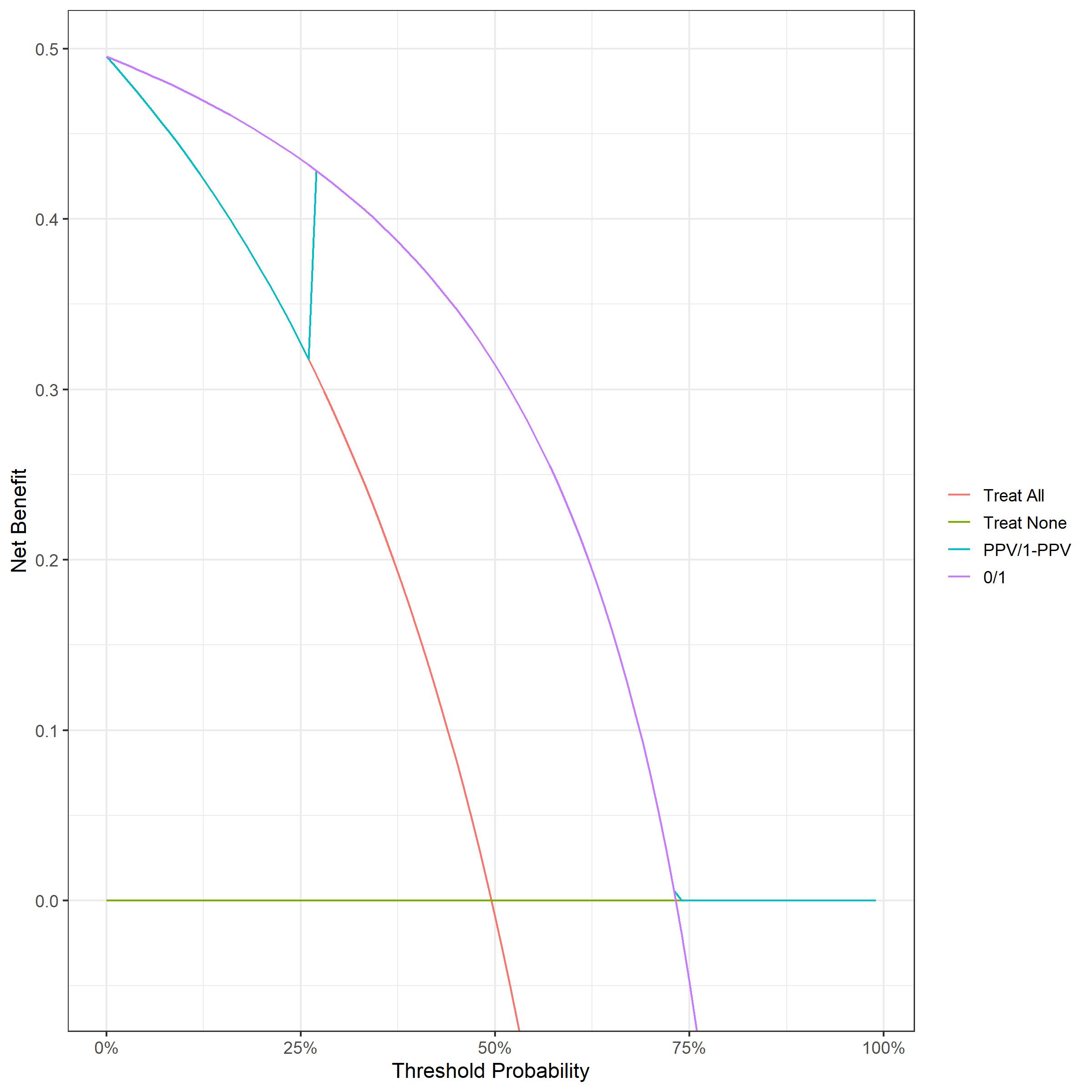
Re the blue line, the example tree has 4 terminal nodes, I’d used the probability for each node rather than overall, which is what you get from the model if you use the ‘predict’ command…
#                 input.dat$nativeSpeaker
# input.dat$node  no yes
#               4 13   0
#               5  0   9
#               6 21   0
#               7 19  43

# probability for node 4 = 0 (0/13)
# probability for node 5 = 1 (9/9)
# probability for node 6 = 0 (0/21)
# probability for node 7 = 0.69 (43/62)

head(predict(output.tree, type = "prob"))

# [[1]]
# [1] 0 1
#
# [[2]]
# [1] 0 1
#
# [[3]]
# [1] 0.3064516 0.6935484
#
# [[4]]
# [1] 0.3064516 0.6935484
#
# [[5]]
# [1] 0.3064516 0.6935484
#
# [[6]]
# [1] 0.3064516 0.6935484
If I use the overall PPV i.e.
cm <- confusionMatrix(input.dat$pred, input.dat$nativeSpeaker, positive = "yes")
ppv <- cm$byClass[3]
ppv
# Pos Pred Value
# 0.7323944

input.dat$prob <- input.dat$pred
input.dat$prob[input.dat$pred==0] <- 1-ppv
input.dat$prob[input.dat$pred==1] <- ppv
I get something more like your example BUT with a step up to meet the purple line at 1-PPV:
Should my purple line cross the treat all line? Looking at the raw data, the test gets all of the positives meaning that the true positive rate is the same for treat all and the 0/1 model, since the weighting at threshold 0 cancels out the false positive rate the net benefit at this point for the two is identical.
Thank you, your time and advice is greatly appreciated!
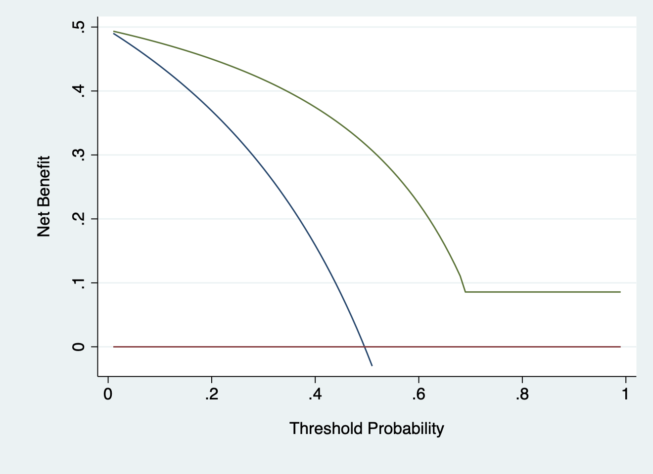
I used your data to get the following graph. I used probabilities of 0, 1, 0 and .96 for nodes 4 - 7, respectively. It has some odd properties (like not crossing treat all or treat none) because you have 100% sensitivity or 100% specificity in certain groups (i.e. nodes 4, 5 and 6). chances are we wouldn’t see this sort of thing on external validation.
Thank you @VickersBiostats
I think this is the same as my original attempt, having thought about it though, should the probability be assigned relative to what the node is predicting for example node 4 is predicting an outcome of ‘no’ so should the probability be 1 i.e. the model correctly classified 13/13?
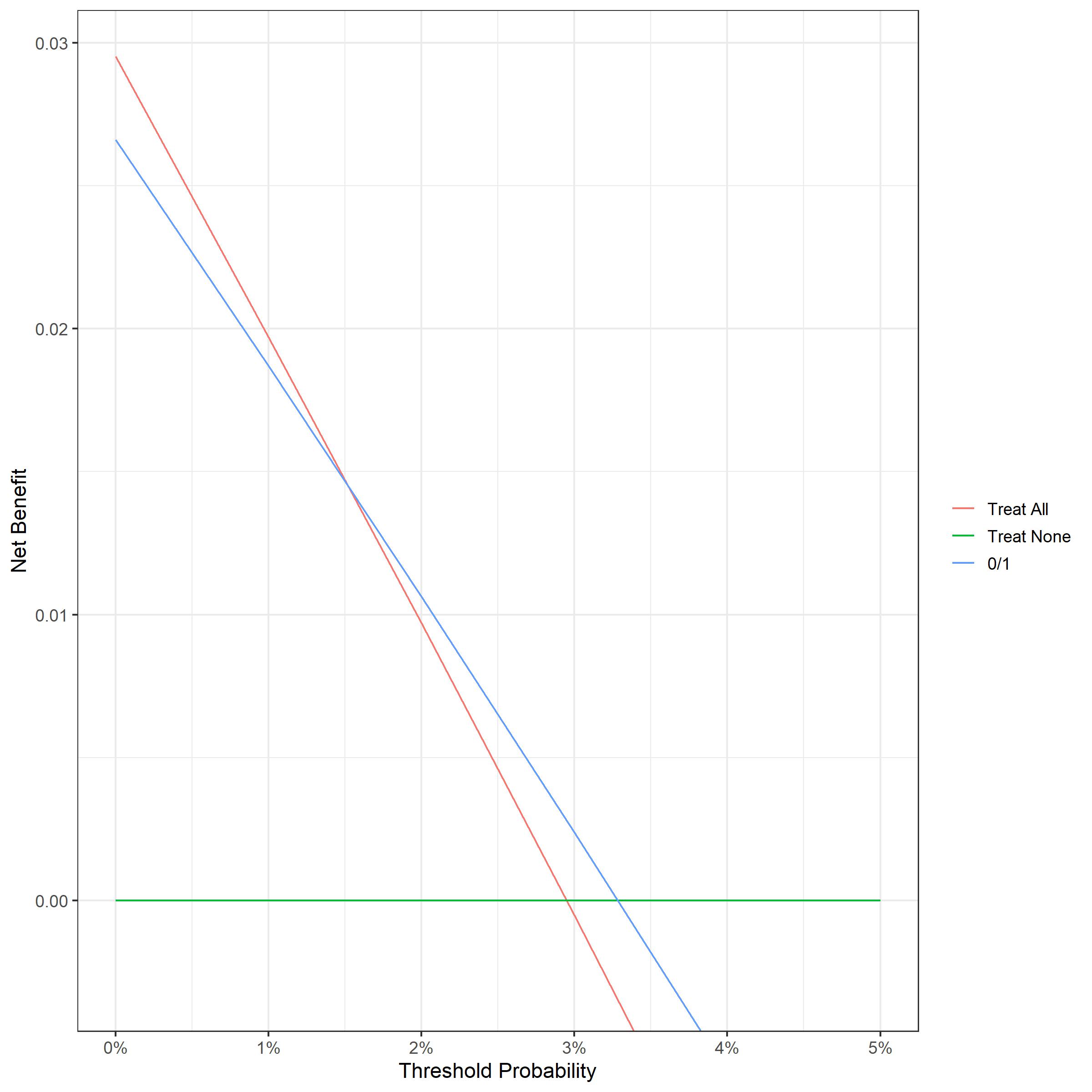
I’ve attached a copy of the curve from my actual data (real life patient data and so unable to share), based on binary 0/1 probabilities.
My model is based on determining which patients to test for a marker of progression to RA.
I’m still struggling to see how I would interpret this given that as you say with a binary test the outcome is either positive or negative and also your comment ‘you don’t apply a threshold in clinical practice’.
Many thanks
The probability is of the event. So if node 4 predicts no event because 13/13 at that node had no event, then probability is 0.
@VickersBiostats thanks!
And what about the interpretation of the curve?