I’m writing a paper about “An Empirical Assessment of the Cost of Dichotomization” together with Frank Harrell (@f2harrell) and Stephen Senn (@Stephen). In this paper, we quantify the information loss due to dichotomization in (clinical) trials, which is also called “responder analysis”. It’s not submitted yet, so we would very much appreciate your comments!
Many statisticians, including Frank and Stephen, have objected to dichotomization, see Categorizing Continuous Variables and Statistical Errors in the Medical Literature: Dichotomania. Unfortunately, so far, this has not had the desired result as the majority of clinical trials continue to have low-information binary outcomes (Figure 2 below). We hope to add some new ways to dissuade clinical researchers from dichtomizing continuous outcomes.
We use of the following mathematical fact (which is not new):
Suppose the continuous outcome has the normal distribution. Then both the standardized mean difference (SMD) and the probit transformation of the dichotomized outcome are estimators of Cohen’s d.
You can see this equivalence in Figure 1 below. We use it to calculate by how much the sample size may be reduced if the outcome would not be dichotomized. We hope that this will motivate researchers during the planning phase not to dichotomize.
We also provide a method to calculate the loss of information after a responder analysis has been done. We hope that this will motivate researchers to abandon dichotomization in future trials.
Finally, we will use 21,435 unique trials from the Cochrane Database of Systematic Reviews to study the loss of information due to dichotomization empirically. We can clearly see that researchers do tend to increase the sample size to compensate for the low information content of binary outcomes, but not sufficiently. We show the loss of statistical power in Figure 5.
Cohen’s d, the SMD and the probit transformation
The Figure below is meant to explain the equivalence between Cohen’s d and the probit transformation. The top panel of the Figure shows two normal distributions with unit standard deviations. The distributions are shifted by some distance d (Cohen’s d). The shaded areas are the probabilities when we dichotomize at some cut-off. The bottom panel shows the associated quantiles of the standard normal distribution. The distance between these quantiles is the probit transformation, which is equal to d. This correspondence does not depend on the choice of the cut-off.
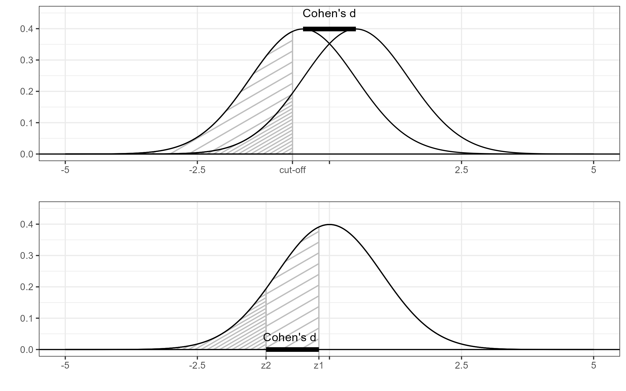
Figure 1 Cohen’s d and the probit transformation.
With the continuous outcome, we can estimate Cohen’s d with the standardized difference of means, which is SMD = \frac{m_1 - m_2}{s}, where m_1 and m_2 are the sample averages and s is the pooled sample standard deviation.
With the dichotomized outcome, we can estimate Cohen’s d with the probit transformation of the responder proportions, which is PBIT = \Phi^{-1}(p_2) - \Phi^{-1}(p_1), where \Phi^{-1} is the quantile function of the standard normal distribution.
Information loss
It is clear that dichotomization causes some loss of information. The extent of this loss depends on the cut-off, with more imbalance between responders and non-responders resulting in a greater loss of information.
If the continuous outcome has the normal distribution, then both PBIT (=the probit transformation of the responder proportions) and SMD are estimating the same population parameter, namely Cohen’s d. Therefore, we can quantify the loss of information by comparing their (sampling) variances. The ratio of the sampling variances is known as the relative efficiency, which we denote by R.
The relative efficiency may be interpreted as the proportion of information that is retained after dichotomization. Hence, 100\% \times (1-R) is the percentage of information lost. R may also be interpreted in terms of a reduction of the sample size. Recall that the sampling variance is inversely proportional to the sample size; if we double the sample size, then the sampling variance is halved. Therefore, the factor by which the sample size would have to be increased to compensate for the loss of information is equal to 1/R.
R is maximal when the numerical observations are dichotomized into groups of equal size and that in that case it is equal to 2/\pi which is approximately 0.64. So, even in the most favorable case, the loss of information due to dichotomization would have to be compensated by an increase in sample size by a factor 1/0.64=1.57.
We do not need the original, continuous outcome to assess the information loss due to dichotomization. The responder proportions in both arms are enough to make an approximation. For example, the CHEST-1 trial had a continuous endpoint. In a follow-up analysis, this endpoint was dichotomized for a responder analysis. After dichotomization, there were 92 responders among 173 in the treated group, and 21 responders among 92 subjects in the control group.
The following R code computes the probit transformation PBIT, its sampling variance, the approximate sampling variance of the SMD and the relative efficiency.
rel_eff = function(events1,events2,n1,n2){
  p1=events1/n1; z1=qnorm(p1)
  p2=events2/n2; z2=qnorm(p2)
  PBIT=z2-z1
  v_PBIT=2*pi*p1*(1-p1)*exp(z1^2)/n1 + 2*pi*p2*(1-p2)*exp(z2^2)/n2
  v_SMD=(n1+n2)/(n1*n2) + PBIT^2/(2*(n1+n2))
  rel_eff=v_SMD/v_PBIT
  data.frame(PBIT,v_PBIT,v_SMD,rel_eff)
}
Running this code, we get
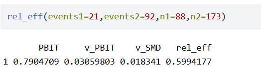
So, the dichotomization effectively caused a reduction of the sample size by a factor 0.6. In other words, the information loss due to dichotomization would have to be compensated by an increase in sample size by a factor 1/0.6=1.67.
Sample Size Calculations
Suppose that somebody is planning a trial where a continuous outcome is to be dichotomized to determine the responders and non-responders to some treatment. In that case, the sample size calculation will be based on the assumed responder probabilities in the two groups.
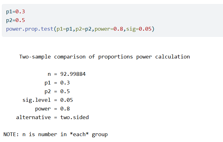
As an example, suppose that we expect the responder probabilities to be p_1=0.3 and p_2=0.5. We calculate the required sample size to have 80% power.
No additional information is needed to also compute the required sample size if the outcome would not be dichotomized. We start by applying the probit transformation to the responder probabilities. Assuming normality, this is the same as Cohen’s d. Therefore we can now run a sample size calculation for a two-sample t-test, setting the difference of means to equal to Cohen’s d and the standard deviation equal to 1. We find
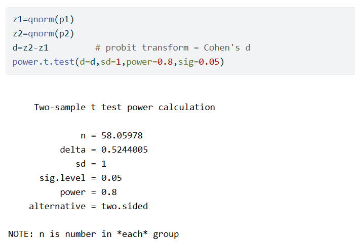
So, in this example, the t-test requires 59/93=0.63 times fewer subjects than the proportions test.
Cochrane Database of Systematic Reviews
The Cochrane Database of Systematic Reviews (CDSR) is arguably the most comprehensive collection of evidence on medical interventions. We use the primary efficacy outcomes of randomized controlled trials (RCTs) from the CDSR. We removed trials with fewer than 10 or more than 1000 participants. Other filtering steps, which may be inspected in the online supplement of the paper, resulted in the primary efficacy results from 21,435 unique randomized controlled trials (RCTs). Of these trials, 7,224 (34%) have a continuous (numerical) outcome and 14,211 (66%) have a binary outcome. This proportion changes over time, but has always been very high. It seems to have reached a minimum around 2010 and then stayed more or less constant (Figure 2).
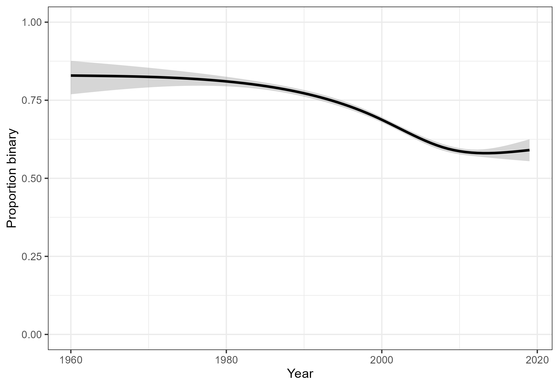
Figure 2: The proportion of trials with a binary outcome.
The median sample size of the RCTs with a continuous outcome is 58 (IQR 33 to 104). For binary trials, the median sample size is 96 (IQR 51 to 197). Among trials with a continuous outcome, 38% are statistically significant. Among those with a binary outcome, 25% are statistically significant. Thus, despite having much larger sample sizes, many fewer binary trials reach statistical significance. This suggests that researchers do increase the sample size to account for the fact that binary outcomes are less informative than continuous ones, but not sufficiently. We will now study this in more detail.
We used natural regression splines with three degrees of freedom to regress the standard error on the square root of the sample size (Figure 3, left panel). We see that for any given sample size, trials with a binary outcome have less information than those with a continuous outcome. We also regressed the binary event whether a trial was statistically significant on the square root of the sample size (Figure 3, right panel). We conclude from Figure 3 that for any given sample size, RCTs with continuous outcomes carry more information and have greater statistical power than those with binary outcomes.
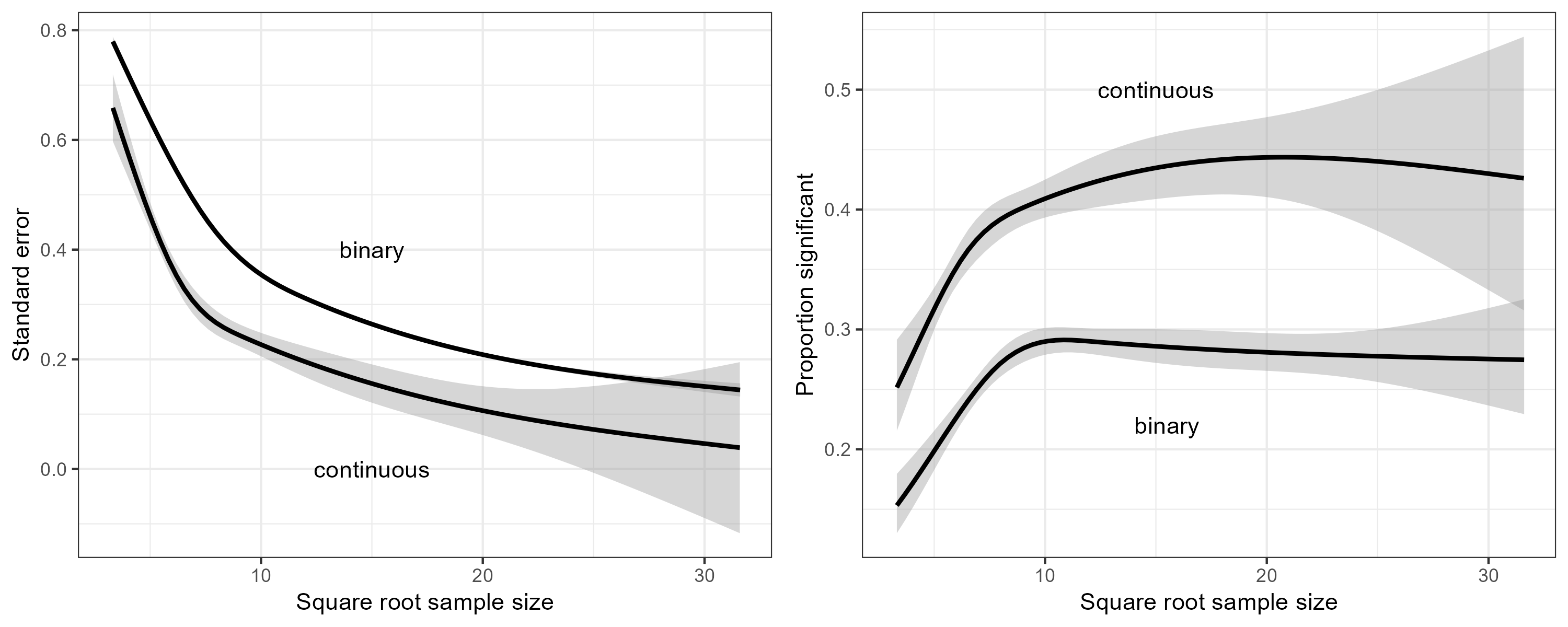
Figure 3: Left panel: The standard error versus the square root of the sample size. Right panel: The proportion of significant trials versus the square root of the sample size.
Next, we used natural regression splines with three degrees of freedom to regress the square root of the sample size on the magnitude of the estimated effect (Figure 4, left panel). This effect is the SMD for the continuous trials, and the PBIT (=probit transformation of the responder proportions) for the binary trials. Similarly, we also regressed the standard error on the magnitude of the estimated effect (Figure 4, right panel). At any given effect size, we see that the average sample size of the binary trials is larger than the average sample size of the continuous trials. However, the increased sample size is not enough; the standard error of the binary trials is still larger on average than that of the continuous trials.
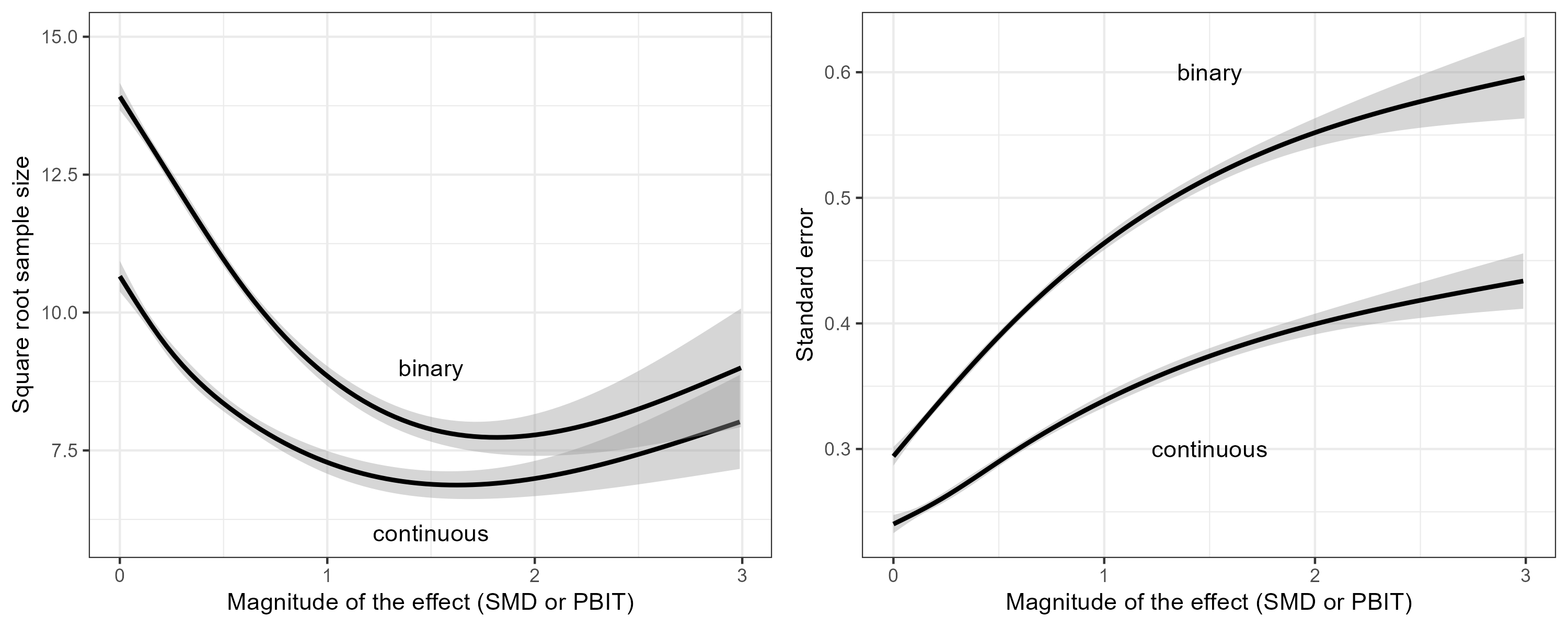
Figure 4: Left panel: The square root of the sample size versus the magnitude of the estimated effect. Right panel: The standard error versus the magnitude of the estimated effect. For trials with a continuous outcome, the effect is the SMD. For trials with a binary outcome, the effect is the PBIT.
Figure 4 demonstrates that researchers do increase the sample size to compensate for the fact that binary outcomes are less informative than continuous outcomes, but not sufficiently. Consequently, trials with binary outcomes have lower power than trials with continuous outcomes. This is demonstrated in Figure 5, where we regressed the binary event whether a trial was statistically significant on the estimated effect size (SMD or PBIT).
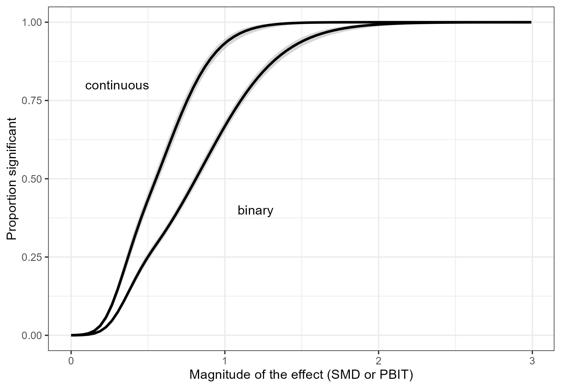
Figure 5: The proportion of significant results versus the magnitude of the effect. For trials with a continuous outcome, the effect is the SMD. For trials with a binary outcome, the effect is the PBIT.
Finally, we used the rel_eff() function from the first part of this blog post to approximate the relative efficiency of all the RCTs with a binary outcome (Figure 6). We find that many trials have a relative efficiency near the statistically optimal value of 0.64. This may indicate that the cut-off is sometimes not chosen for clinical relevance, but rather to limit the loss of statistical power. There are also many trials where the responders and non-responders are not well balanced, and consequently the loss of information is much greater.
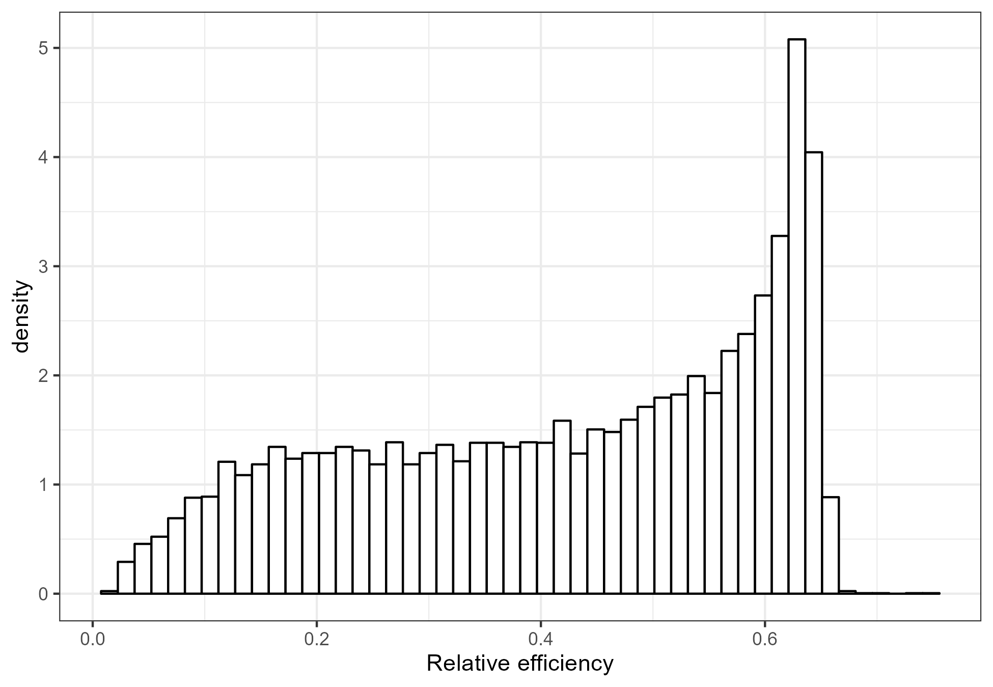
Figure 6: The distribution of the relative efficiency of the trials with a binary outcome from the CDSR.
The information loss we see in Figure 6 is all the more serious as two thirds of the randomized trials in the CDSR have a binary outcome as the primary efficacy endpoint. Of course, not all trials with a binary outcome result from dichotomization of a continuous outcome. However, if a trial does involve dichotomization, then the loss of information is avoidable.
Discussion
It is believed by some that categorization of noisy continuous variables reduces measurement error. In fact, the opposite is true. For example, a systolic blood pressure (SBP) threshold of 140 mmHg leads to classification of an observed SBP of 141 mmHg as hypertensive. If the true SBP were actually 139 mmHg, the resulting misclassification represents an error of the worst kind. A continuous analysis would also be affected, but not nearly as much (just by 141 versus 139).
The magnification of the noise around the cut-off is part of the reason why dichotomization leads to a loss of information. The other part is that all measurements above (or below) the cut-off are lumped together. For example, the difference between 141 mmHg and 180 mmHg is lost. The latter is referred to as a “hypertensive crisis” which is a medical emergency.
Some have argued that dichotomization leads to effect sizes (such as risk differences, numbers needed to treat, risk ratios and odds ratios) that are clinically more relevant or more easily interpreted than the effect sizes associated with continuous outcomes (such as difference of means or standardized difference of means). We do not find this argument compelling, but ultimately the question of clinical relevance and ease of interpretation may remain a matter of opinion. The empirical evidence from the CDSR, however, is unambiguous. It is quite clear that trials with binary endpoints have larger sample sizes on average than trials with continuous endpoints, while a lower proportion reaches statistical significance.