Hi everyone,
I’m trying to replicate the plot of relative hazard over age by sex from this vignette from the survival package. However, I notice a difference in the confidence intervals (CIs) around the relative hazard estimates depending on how I compute them.
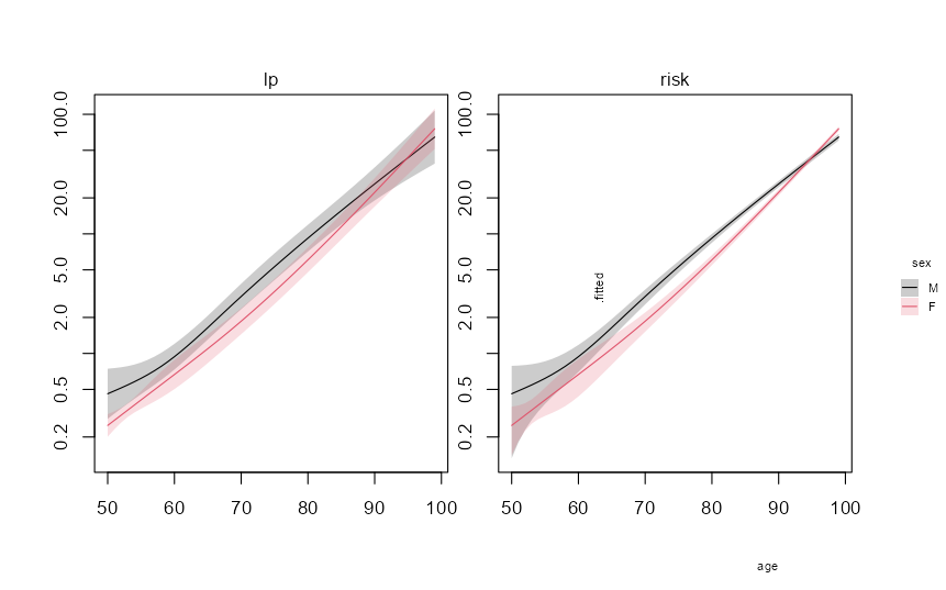
Specifically, I obtain different CIs when using:
type = "lp"inpredict(), then computing the 95% CI from the standard error (SE) and exponentiating the results (as done in the vignette).type = "risk"inpredict(), then computing the 95% CI directly from the SE.
The confidence interval is narrower in the second case.
According to the help file of predict.coxph, "risk" is simply exp(lp), so I would have expected the two approaches to yield the same results.
Does anyone have an idea why they differ?
Thanks in advance for your insights!
library(survival)
library(dplyr)
library(tinyplot)

fit <- coxph(Surv(futime, death) ~ sex * splines::ns(age, df =3), data = flchain)
pdata <- expand.grid(age = 50:99, sex = c("M", "F"))

lp_pred <- broom::augment(fit, newdata = pdata, type.predict = "lp", se = TRUE) |>
  mutate(
    type = "lp",
    conf.low = .fitted - 1.96 * .se.fit,
    conf.high = .fitted + 1.96 * .se.fit,
    across(c(.fitted, conf.low, conf.high), exp)
  )

risk_pred <- broom::augment(
  fit, newdata = pdata, type.predict = "risk", se = TRUE
  ) |>
  mutate(
    type = "risk",
    conf.low = .fitted - 1.96 * .se.fit,
    conf.high = .fitted + 1.96 * .se.fit
  )

pred <- rbind(lp_pred, risk_pred)

with(
  pred,
  tinyplot(
    x = age, y = .fitted, ymin = conf.low, ymax = conf.high, by = sex,
    facet = type, type = "ribbon", log = "y"
  )
)