I think that is correct.
1 Like
This is an older discussion on the blog article page, from the previous web platform for the blog, from 2019.
Ewout Steyerberg: Great illustration of detailed modeling in a large-scale trial!
One question on the choice of penalty. The AIC seems to be optimal with penalty going to infinity, so no interactions? What is the basis for the choice of penalty = 30000:
h <- update(g, penalty=list(simple=0, interaction=30000), ...)
Is this merely for illustration of what penalized interactions would do?
Frank Harrell: Thanks Ewout. Yes by AIC the optimum penalty is infinite. I overrode this to lambda=30000 to give the benefit of the doubt to differential treatment effect. It would be interesting to see in a Bayesian analysis would result in the same narrow distribution for ORs.
1 Like
@f2harrell have you explored these distributions of ARRs in the Bayesian context? In this case, one would have a posterior distribution for each ARR, which is quite difficult to visualize/summarize.
I know @BenYAndrew has nicely developed a shiny app to show each patient-specific ARR separarely. Bayesian Modeling of RCTs to Estimate Patient-Specific Efficacy
Thanks for circling back on this, @arthur_albuquerque. After some of our discussions I’ve continued to play around with this. Here is one approach at summarizing these data:
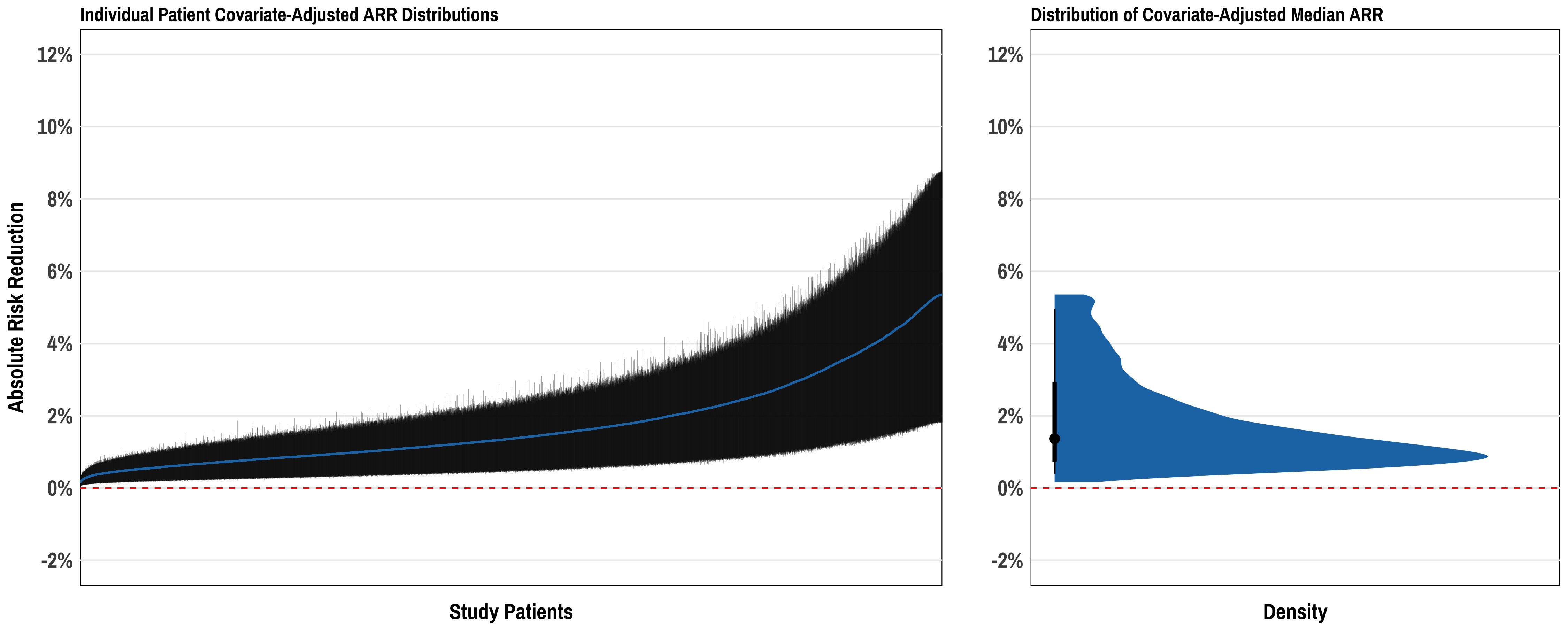
Here the left plot is a set of >10,000 patients from an example dataset with each patient represented by her/his median ARR +/- 95% credible interval. This shows the “distribution of distributions” so to speak, of ARRs across the range of patients in the cohort. The right plot shows the distribution of median ARR for the study cohort, distilling each patient’s covariate-adjusted ARR to its median value across all posterior draws. Not sure this is the “right answer” - but just a thought. The third piece to all of this could be then displaying the distributions of actual patient-level predicted ARR for various representative patients (similar to the Shiny app you reference above).
1 Like
This is really excellent. For the very particular case of estimating a probability, the posterior mean may be slightly better than the posterior median.
The width of the posterior distribution for one patient’s ARR is a function of how close the posterior mean is to 0.5 and a function of the covariates, the latter related to the distance of covariates from their means. It may be useful to get 10 or so representative patients over the distribution of these two metrics and to present their posterior densities to accompany the left panel above.
1 Like
Hi Dr. Harrell,
I saw that you linked the {marginaleffects} vignette to your blog post Statistical Thinking - Avoiding One-Number Summaries of Treatment Effects for RCTs with Binary Outcomes
A couple of notes:
- The link is broken. This is the correct one now: Logistic Regression • marginaleffects
- I wrote the vignette and Vincent edited.
Thanks!
1 Like
Fixed - thanks for alerting me.
1 Like
Hi @f2harrell,
A new RCT just published on JAMA applied a causal forest method to estimate conditional average treatment effects at the levels of the individual (Figure 3B).
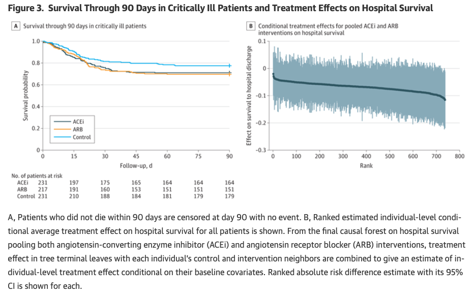
It reminded me of these plots in your work:
Would you mind discussing potential advantages or pitfalls of causal forests vs. your approach? Thanks.
I need to understand what right the authors had to put the word causal on this method. As far as I can tell, it’s the usual “assume we have the needed confounders measured” analysis, so under that unverifiable assumption you can conclude the effects are caused by the intervention. I’m not convinced that this is safe.
I think the method ends up being a very complex, harder to understand version of what I did. I’m open to being corrected.
Then there is the extreme overfitting we see in so many random forest applications. Almost every application I’ve seen of random forests either has a bad result, no advantage over simpler methods, or the authors failed to do the assessment needed to see if the result is bad (overfitting, over-interpretation).
And the authors’ belief (in the ArXiv paper at least) that the method can pull information about treatment effect heterogeneity out of thin air when the sample size does not support the estimation of differential treatment effects.
2 Likes
I’ve been thinking about how to apply this method when a trial includes multiple follow-up intervals. A typical way that one could analyse such a trial would be to use a multilevel model with random intercepts for subjects and a group by time interaction to estimate group differences at each follow-up interval.
Assume that we want to predict the outcome for a subject if they had been randomised to the control arm rather than the intervention arm. It seems natural to me to use all the information available and include this subject’s estimated intercept when making predictions of outcomes at each follow-up interval. For me this is what we mean by counterfactual arguing, i.e. conditional on that I have seen outcome Y = y_1 when X = 1, what value would Y have taken if X = 0.
But what about when I want to evaluate the predictive capacity of the model? If I take a cross-validation approach and split my long data into folds, then it is possible that I get data for a subject both in the estimation and validation folds (i.e. data for two different follow-up intervals). If the goal is to “predict for a new individual”, then this would be cheating since I should not have any data for this individual. But when it comes to this counterfactual prediction I’m not “predicting for a new individual”, I’m using all information available to predict something about an individual I have already studied. This is akin to how one uses auxiliary variables when using multiple imputation with chained equations.
Of course, an easy way to get around this is to define CV folds on subjects rather than data points. But this will severely underestimate the predictive power of the model that I am actually going to use to do the counterfactual predictions, which is allowed to “remember” something about the individual through the random intercept (and so it may be an unfair evaluation of the method).
So my question is really: Should a model used to predict individual level response be shown to be able to do out-of-sample predictions to some degree of acceptability (e.g. RMSE, calibration, etc.), or should we evaluate these models more like we would when doing imputation, when auxiliary information is recommended?
Thanks in advance!
It may be easier to start with a situation where the sample size is so large that cross-validation isn’t needed, and see if you can estimate what you need. In general, random effects models may not capture the true serial correlation structure (that’s clear for random intercepts; not sure what correlations are assumed by random slopes) and other methods of handling correlation are needed. But once the correlation structure is well-modeled, the meaning of the random effects needs close examination. I don’t think they can be used to derive “what if this patient had recieved the alternate treatment” as needed for causal inference.
1 Like
Thank you @f2harrell - I think that this helps me to get my head around this partially. I’m still pondering if individual treatment effects (which requires some form of prediction because we only see each participant under one condition and not the other) should be thought of as an out of sample prediction problem where we should only use data that was available at the time of randomization, or more akin to imputation which I think of as an within sample prediction problem (albeit with purposefully added noise) were we use any data that we have to “fill in the blanks”.
Leaving out some observations helps with estimation of uncertainties, but our best estimates of outcome tendencies comes from using all the data.
Thank you again - that gives me a succinct way of resolving this chain of thought !