Quite a while ago I attended a conference talk on sensitivity analysis with multiple confounders. The talk is archived and can be accessed here:
http://www.sfu.ca/~lmccandl/LectureACIC.pdf
There was one small aspect of the talk that caught my attention:
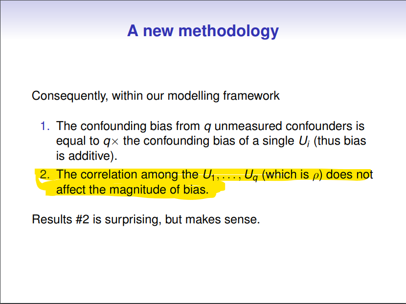
the claim that the correlation between confounders is completely irrelevant for the amount of bias.
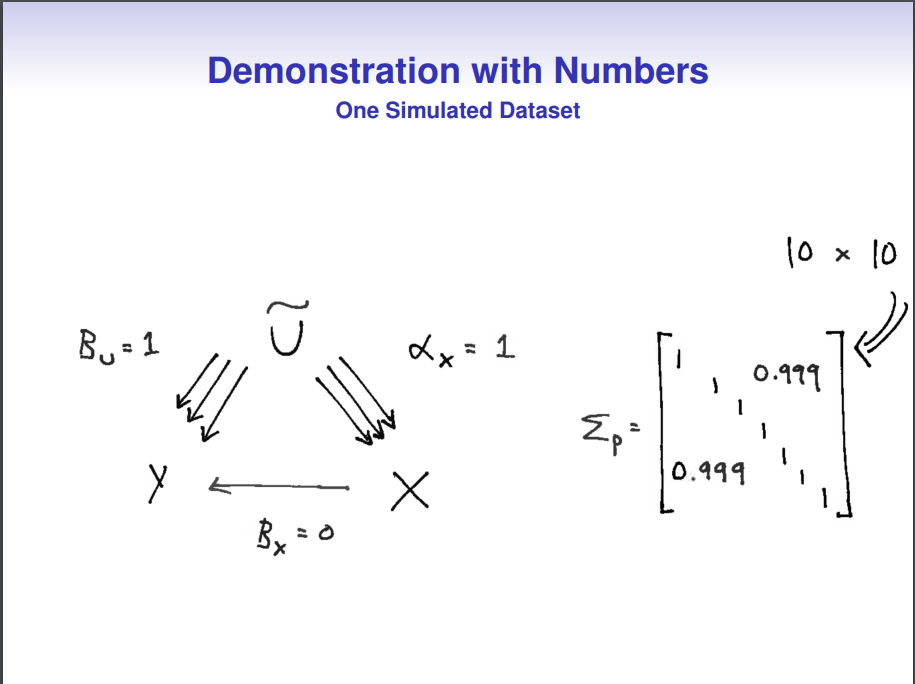
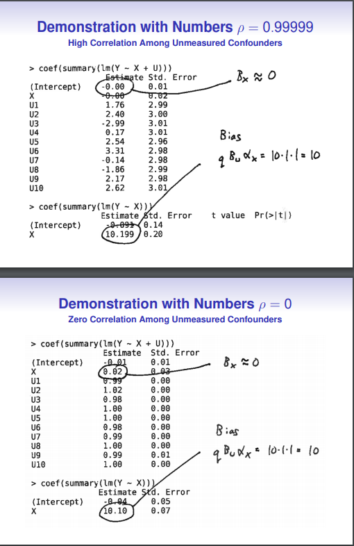
I am copying the relevant four slides from the presentation here:

Back then I was quite surprised by this result, because it went counter to my intuition. I tried to talk to the author, and to some other folks at the conference, but everybody seemed to agree with the presenter.
Even though the original author used 10 correlated covariates in the example, I am using only two to make the equations a bit easier.
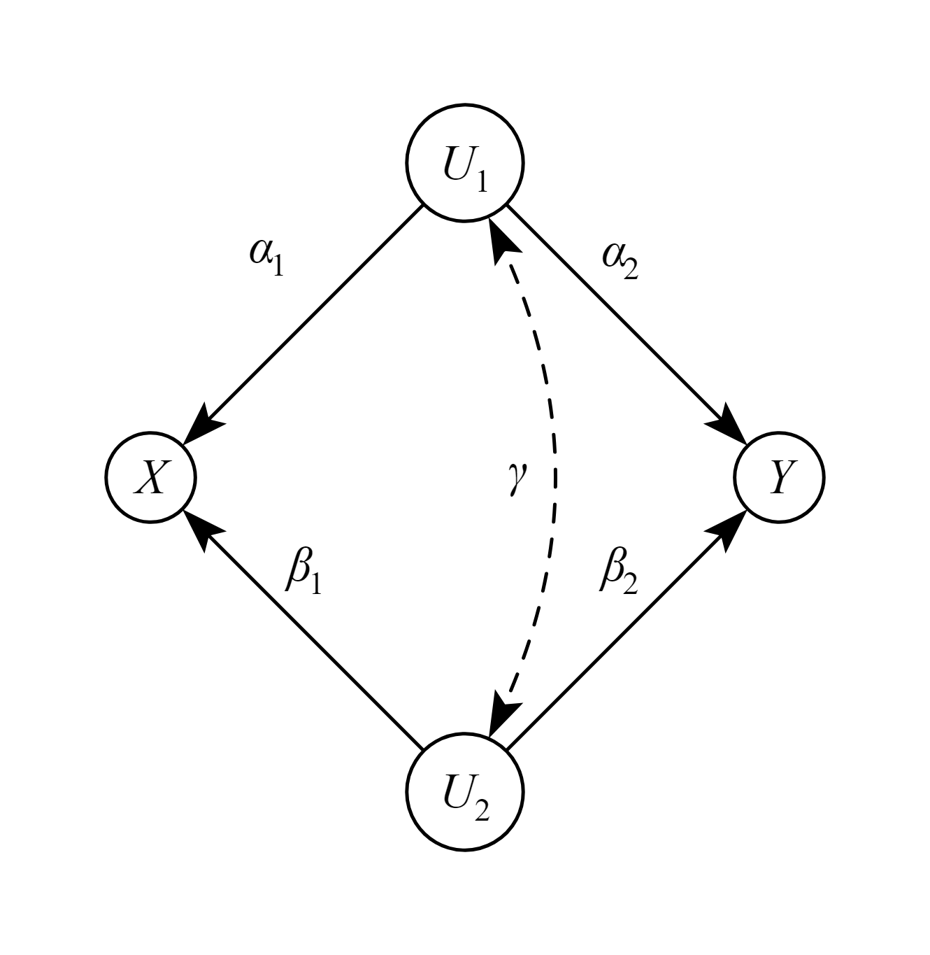
When I considered the bias of the causal effect between X and Y in the DAG above, I simply assumed all standardized variables, and then following Wright’s tracing rules, and Pearl , I get as the bias in the DAG above:
bias = \alpha_1\alpha_2 + \beta_1 \beta_2 + \alpha_1 \gamma \beta_2 + \beta_1 \gamma \alpha_2
In DAG language, I simply added up all open back-door path. And here we see that the correlation between the confounders indeed changes the amount of bias. If \gamma is zero, then bias is simply a function of the \alpha 's and \beta 's, but as soon as \gamma is non-zero, bias can either increase or decrease depending on the signs of the back-door path coefficients.
In order to reconcile this with the results from the presenter, I simulated some data using the code provided on his slides, and own R code. I simulated different correlations between the confounders, but I left the influence of the confounders themselves (\alpha, \beta) constant across all simulations.
In one simulation which I call constant error, I fixed the residual (error) terms of all endogenous variables to be always 1.0 (using rnorm(n,0,1) in R). In another simulation, which I call constant marginal variance, I fixed the residual terms of all endogenous variables in such a way that the TOTAL variance of each variable is always 1.0, regardless of any path coefficients. This typically meant reducing error variance in proportion to influence from other variables. Given that the mean of all variables is always zero, we could also call this scenario “z-score standardized variables”. Lastly, I used the R code from the slides, in which I noticed that the variance of the outcome Y is unbounded and not fixed, and increases in proportion to the influence of the unobserved confounders.
I plotted results of this simulation
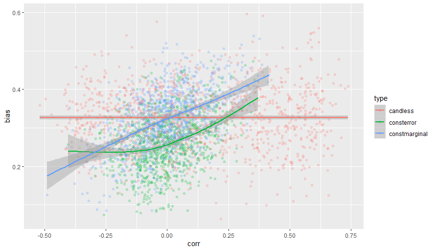
The red line stands for the simulation of the original presenter, and it is indeed completely flat, indicating that bias is independent of the correlation among confounders.
The other two scenarios show that correlation between confounders does matter, and the bias (for standardized variables, blue line) can be derived by the formula that I gave above.
My questions:
1) does the correlation between confounders have an influence on the magnitude of overall bias?
2) which way to simulate data is appropriate? Constant total variance, constant error variance, or let variances be whatever they like, and just focus on coefficients?
Thanks for any comments and insights!
R code appended for reproducible results:
library(tidyverse)

cor_conf <- function(gamma1, gamma2, alpha1, beta1, alpha2, beta2, correl, n) {

  #data-generation in which error (residual variance) is always constant at 1 for all vars
  uu <- rnorm(n,0,1)
  epsu1 <- rnorm(n,0,1)
  epsu2 <- rnorm(n,0,1)
  epsx <- rnorm(n,0,1)
  epsy <- rnorm(n,0,1)
  u1 <- gamma1*uu + epsu1
  u2 <- gamma2*uu + epsu2
  x <- alpha1*u1 + beta1*u2 + epsx
  y <- alpha2*u1 + beta2*u2 + epsy

  consterrorcor <- cor(u1,u2)
  consterror <- lm(y ~ x)$coef[2]

  #data-generation in which total variance is always constant at 1 for all vars (standardized)
  uu <- rnorm(n,0,1)
  epsu1 <- rnorm(n,0,sqrt(1-gamma1^2))
  epsu2 <- rnorm(n,0,sqrt(1-gamma2^2))
  epsx <- rnorm(n,0,sqrt(1-alpha1^2-beta1^2-2*gamma1*gamma2*alpha1*beta1))
  epsy <- rnorm(n,0,sqrt(1-alpha2^2-beta2^2-2*gamma1*gamma2*alpha2*beta2))
  u1 <- gamma1*uu + epsu1
  u2 <- gamma2*uu + epsu2
  x <- alpha1*u1 + beta1*u2 + epsx
  y <- alpha2*u1 + beta2*u2 + epsy

  constmarginal <- lm(y ~ x)$coef[2]
  constmarginalcor <- cor(u1,u2)


  #data-generation in which total variance and error variance of Y are not constant (McCandless)
  #original shared R code with the following minor modifications
  #dimension was intially set to 10, I set it to 2
  #the coefficients alpha1 and alpha2 below were set to 1.0 in original code, for comparison I set them to alpha1,2
  k <- 2 ## Dimension of U
  sigma <- matrix(correl, nrow=k, ncol=k); diag(sigma) <- 1
  X <- rnorm(n, 0,1)
  U <- alpha1*X + matrix(rnorm(k*n), nrow=n, ncol=k) %*% chol(sigma)
  Y <- rnorm(n, 0*X + apply(alpha2*U, 1, sum), 1)

  candless <- lm(Y ~ X)$coef[2]
  candlesscor <- cor(U)[2,1]
  res <- c(consterror,constmarginal,candless,consterrorcor,constmarginalcor,candlesscor)
}


#run simulation with random parameters
res1 <- replicate(1000,cor_conf(runif(1,-.6,.6),
                                runif(1,-.6,.6),
                                .4,
                                .4,
                                .4,
                                .4,
                                runif(1,-.6,.6),
                                200),simplify = TRUE)
res1df <- data.frame(t(res1))
names(res1df) <- c("consterror","constmarginal","candless","consterrorcor","constmarginalcor","candlesscor")

res1dflong <- gather(res1df[,1:3],key="type",value="bias")
corrs <- gather(res1df[,4:6], value="corr")
res1dflong$corr <- corrs$corr


ggplot(res1dflong,aes(x=corr,y=bias,color=type)) + geom_point(alpha=.2) + geom_smooth()