Hello everyone,
So @f2harrell suggested I moved a Twitter discussion on using Bayesian update for interpretation of clinical trials to datamethods. I am a little bit concerned that my code and concepts may not be polished enough, but I will give it a shot. Please correct me if I am wrong, if I could have done this using different methods, etc. Keep in mind I am a regular ICU physician, so I cannot work with more than 4 Greek letters neither understand complex formulas.
The idea, overall, is simple. So simple it may be wrong, so the idea here is to open discussion on this subject.
The FLASH randomized controlled trial will serve as working example. FLASH randomized 775 patients to receive either saline or hydroxyethyl starch (HES) as default fluid during major surgery. It had a binary composite endpoints ([FLASH]). In brief, primary endpoint (which has harmful for the patient) occurred on 36% of HES patients and 32% of saline patients. This ended up as being “negative” and the authors presented a default conclusion.
The idea here is to reinterpret data knowing nothing more than a 2x2 table. No individual data. We will use a beta binomial distribution, since it is easy to update given data. Beta-binomial is cool.
- The authors estimated primary outcome would occur on ~25% of all patients, so it makes sense to center our prior on it. I will consider that a standard deviation of 5% is reasonable here so the prior is not too strong, but any other prior could be used. Don’t blame me. First step is to find parameters alpha and beta on a beta distribution that are compatible with a mean = 0.25 and sd = 0.05:
set.seed(123) library(MASS) library(tidyverse)
#Note to non-statisticians: Beta distributions have alpha and beta parameters so this may be confusing #at first. R calls them shape1 and shape2.
#You will get some NaN messages because sometimes the rnorm will return negative values
#that cannot be used by fitdstr
set.seed = 123
fake <- rnorm(1000,mean = 0.25,sd=0.05)
m <- MASS::fitdistr(fake, dbeta, start = list(shape1 = 1, shape2 = 10)) #gets parameters for beta binomial compatible
alpha0 <- m$estimate[1] #Extract the prior alpha for the beta prior
beta0 <- m$estimate[2] #Extract the prior beta for the beta prior
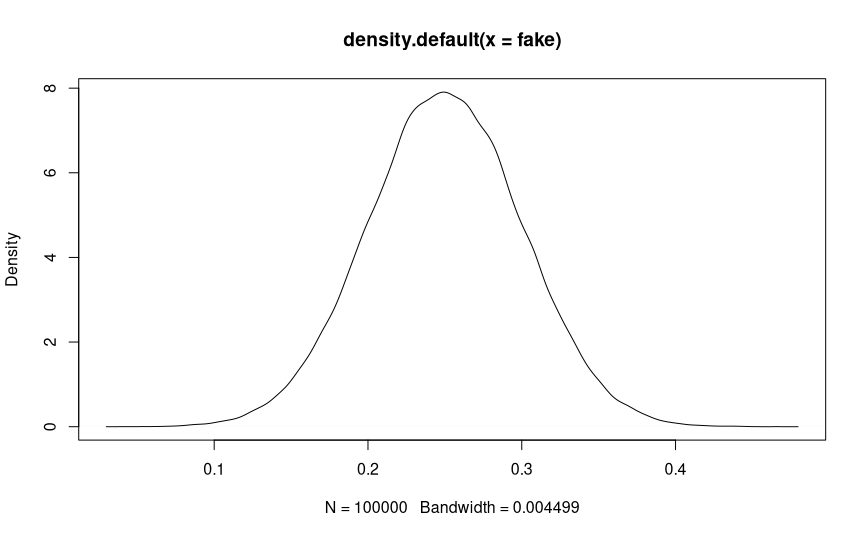
- Cool. So our prior is defined as B(18,53). How does it look?
plot(density(rbeta(1000,shape1=alpha0,shape2=beta0)))
- Next we will update the prior. Saline group had 389 patients, 125 event, 264 non-events. HES has 386 patients, 139 event, 247 non-events. Bayesian updating for Beta looks simple.
alpha.saline <- alpha0 + 125 #adds events to alpha shape for saline
beta.saline <- beta0 + 264 #adds non-events to alpha shape for saline
alpha.hes <- alpha0 + 139 #adds events to alpha shape for HES
beta.hes <- beta0 + 247 #adds non-events to alpha shape for HES
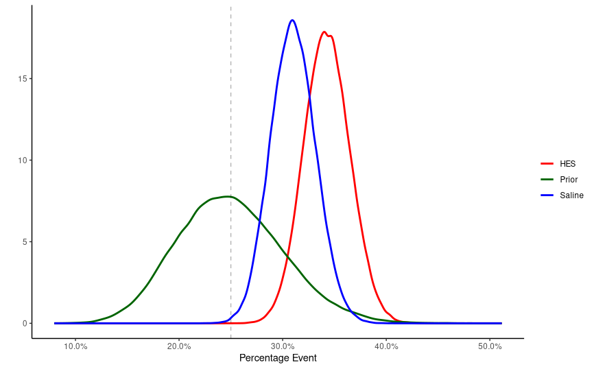
- Time to sample! So now we know three distributions: (1) Prior; (2) Saline; (3) HES. We can just sample using built in R functions to get a data frame of, say, 10^5:
db<- tibble(prior=rbeta(10^5,shape1 = alpha0,shape2 = beta0),
hes=rbeta(10^5,shape1=alpha.hes,shape2=beta.hes),
saline=rbeta(10^5,shape1=alpha.saline,shape2=beta.saline),
dif1=hes-saline)
- Plotting time! Let’s see how this goes. Some wrangling to make it pretty:
db %>%
select(-dif1)%>%
gather(g,vals)%>%
ggplot(aes(x=vals,color=g))+
geom_line(stat="density",size=1)+
scale_color_manual(name="",labels=c("HES","Prior","Saline"),values=c("red","darkgreen","blue"))+
geom_vline(xintercept=0.25,linetype=2,alpha=0.3)+
scale_x_continuous(labels=scales::percent)+
labs(x="Percentage Event",y="")+
theme_classic()
- And what about the difference?
ggplot(db,aes(x=dif1))+ geom_line(stat="density")+ geom_vline(xintercept=c(-0.1,-0.05,0,0.05,0.10),linetype=2,alpha=0.3)+ theme_classic()+ scale_x_continuous(labels=scales::percent)+ coord_cartesian(xlim=c(-0.20,0.20))+ labs(x="Difference HES - Saline",y="")

-
Keep in mind that db$dif1 is a subtraction of two Betas. Although there must be a mathematical way to do so, I googled a bit and found out that it is hard for someone with little math background (as I am). In this particular scenario you could do some assumptions and operations considering only normal distributions, but the idea here is to show how sampling is useful! We can ask db$dif1 lots of cool things!
-
What is the chance it is below zero (HES is bad)?
sum(db$dif1>0) / nrow(db)*100 #This returns 85.2%
- What is the change HES benefit is 10% absolute reduction in primary endpoint? This was the trial hypothesis.
sum(db$dif1 < -0.1) / nrow(db)*100 #This returns something like 0.001% (yes, %)
To wrap up, with some few code which I hope is correct you can interpret binary outcome trials in a simple way. Myself and @larsms are planing to write a wrapper function, maybe a package, on this one day.
Thanks!