I’m helping plan an RCT with a new peri- and postoperative treatment protocol as the intervention.
The outcome is a composite score representing complication severity (from 0=nothing to 100=worst).
The score validation study show this distribution of scores:
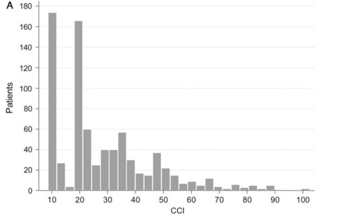
Our potential participants seem to have a similar distribution.
The current analysis plan is to fit this regression model:
lm(log(Outcome_score) ~ Treatment + Surgery_open)
Where treatment is the intervention and Surgery_open indicates open vs closed surgery which is a known risk factor.
The problem is that this model assumes that the treatment effect is relative. We actually believe that it will be absolute (e.g. 10 points), but of course have a flooring effect.
If we omit the log transform, the expected values should behave as we want, but the residuals will be highly skewed (surgery type can only explain a small part of the variance).
Any suggestions for a model that will allow us to estimate an absolute effect of treatment and also fit this highly skewed data?
(Another problem with the log-transform is that the lower scores are clustered at values of e.g. 0(1), 8 and 20, making a lot of the effect hinge on whether the treatment can move a few patients from e.g 8 to 1).
I think absolute treatment effects on bounded scales are hard to defend since when we meta-analyse these the estimates tend to be so heterogeneous across studies/the model requires (and in some ways assumes the existence of) interaction effects. If you’re dead set on the idea you could always resort to OLS with robust errors a la econometrics. Another solution would be to separate the idea of how you model the data vs how you summarize effects and use something like a proportional odds model with post-hoc summaries of mean difference or exceedance probabilities, etc. If you are more of the data-generating process type and it would be important to predict scores (including those that haven’t been seen in your analysis) then you could look at zero-one inflated beta with the same post-processing idea.
2 Likes
I’m not that set on the absolute treatment effect. I’m mainly afraid that the relative treatment effect will put a lot of weight on the changes in the bottom of the scale.
I think I’m the data-generating process type  Not because I need the predictions, but because I understand the parameters if I understand the data-generating process. I’ll have to look more into post-hoc summaries.
As @timdisher suggested, a semiparametric ordinal response model such as the proportional odds model (a generalization of the Wilcoxon test) is highly likely to work well here. It will handle arbitrarily high clumping at one end and any other distribution oddities. You can use the model to estimate means, medians, and differences and ratios of these. The primary model parameters provide odds ratios for Y \geq y between two groups, for all y, and cumulative probabilities for all Y \geq y and concordance probabilities.
One big problem with the use of the log transform is that it needs to be \log(Y + \epsilon) and we don’t know how to choose \epsilon. You automatically assumed that \epsilon=0 and this is unlikely to be correct. With semiparametric models the results are invariant to transformations of Y until you get to the point of estimating means. A detailed case study is in RMS and an introduction to the proportional odds model may be found in the Nonparametrics chapter of BBR.
2 Likes
Thank you. I’ll see if I can analyse my simulated study with a proportional odds model.
I’m not sure why the log transform assumes that \epsilon = 0. I thought that it would just assume that \epsilon \propto Y.
I tried fitting a proportional odds model using rms::lrm(). I post the result below, but I’m unsure how I can use this model to estimate the between group difference (absolute or relative), and not just the odds ratios as shown below.
library(rms,quietly = TRUE)

library(ggplot2)

# Let me know if there is a more appropriate way to share data.
sim <- readr::read_csv("https://gist.githubusercontent.com/JohannesNE/5812d1e99998524e23f8200af46b6eb6/raw/689109d34f03be509b786586e1e683eec3c75eab/simulated_data.csv",
                       col_types = "dcc")
sim$cci_f <- ordered(sim$cci)

dd <- datadist(sim)
options(datadist="dd")

ggplot(sim, aes(cci_f, fill = treatment)) +
    geom_bar(position = position_dodge(preserve = "single"), width = 0.8)
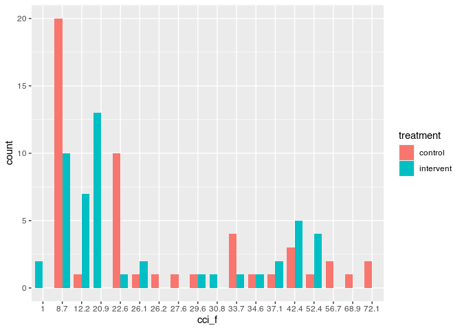
po_mod <- lrm(cci_f ~ treatment + surgtype, data = sim)
summary(po_mod)
#>              Effects              Response : cci_f
#>
#>  Factor                        Low High Diff. Effect   S.E.    Lower 0.95
#>  treatment - intervent:control 1   2    NA    -0.12170 0.35706 -0.82152
#>   Odds Ratio                   1   2    NA     0.88541      NA  0.43976
#>  surgtype - closed:open        2   1    NA    -1.16450 0.37576 -1.90100
#>   Odds Ratio                   2   1    NA     0.31207      NA  0.14942
#>  Upper 0.95
#>   0.57812
#>   1.78270
#>  -0.42804
#>   0.65178
Created on 2022-02-18 by the reprex package (v2.0.0)
I am sure there are clever analytic ways to calculate what you need but normally when I do this it would bayes so I’d create a dataframe where everyone is 0 and a second where everyone is 1 and either use predict (and hope it has function to spit out fitted values for every patient at every sample) or do the same thing manually. In both cases the mean difference would just be mean(predict_trt) - mean(predict_control).
A simpler solution at this phase (and equally brute force) would just be to do the same but with bootstrap. Probably errors in below and I’m assuming predict works as I described above but the general idea:
samps ← purrr::map(1:100, ~ {
bs ← dplyr::sample_frac(sim, replace = TRUE)
trt ← bs > dplyr::mutate(treatment = 1)
ctrl ← bs > dplyr::mutate(treatment = 0)
m ← lrm(cci_f ~ treatment + surgtype, data = bs)
t_pred ← predict(m, newdata = trt, type = “response”)
ctrl_pred ← predict(m, newdata = ctrl, type = “response”)
mean(t_pred) - mean(ctrl_pred)
}) > dplyr::bind_rows
quantile(samps, prob = c(0.025, 0.5, 0.975)
That might work (or at least give the general idea) to just get a sense whether you like the approach to the model. Quantile bootstraps are not great so if you go this route I’d spend some time converting it to format accepted by one of Rs bootstrap packages.
You are forcing \epsilon to be zero since you are using \log(Y + \epsilon) where \epsilon=0. I would expect a negative \epsilon to be need in your case. This just points out the arbitrariness of the log transform unless the variable being transformed is a ratio.
Concerning computations, rms:::orm is more intended for continuous Y. And it has methods to help you get what you want including the Mean function and the ability to get bootstrap confidence intervals for the mean (and for quantiles). See the detailed case study in the “ordinal analysis of continuous Y” chapter in RMS. If you used a Bayesian model using rmsb::blrm things work even better. There is an extensive vignette for here.
@timdisher "response" is not implemented in predict.lrm.
2 Likes
By trying to apply the analysis shown in RMS for the bmi analysis, I get these predictions:
mean_f <-  Mean(po_mod)
Predict(po_mod, treatment, fun = mean_f, conf.int = 0.95)
#>   treatment surgtype     yhat    lower    upper
#> 1   control     open 28.32845 22.81180 33.84509
#> 2 intervent     open 27.20010 21.96793 32.43227
#>
#> Response variable (y):
#>
#> Adjust to: surgtype=open
#>
#> Limits are 0.95 confidence limits
This seems reasonable. I hoped to do the same with contrasts, but it does not seem to work.
contrast(po_mod, list(treatment = "intervent"), list(treatment = "control"),
         fun = mean_f)
#>   surgtype   Contrast      S.E.      Lower    Upper     Z Pr(>|z|)
#> 1     open -0.1217006 0.3570564 -0.8215182 0.578117 -0.34   0.7332
#>
#> Confidence intervals are 0.95 individual intervals
contrast only implements the calculation of contrasts on the mean scale for Bayesian model fits from blrm. The only way I know to get the contrast you want is by more manually programming the bootstrap so that the loop runs orm and Mean and you compute the difference in means once per iteration.
1 Like