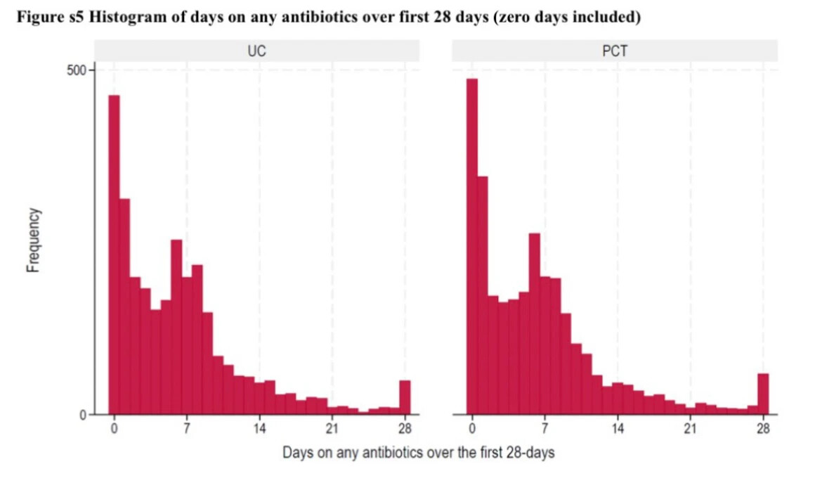
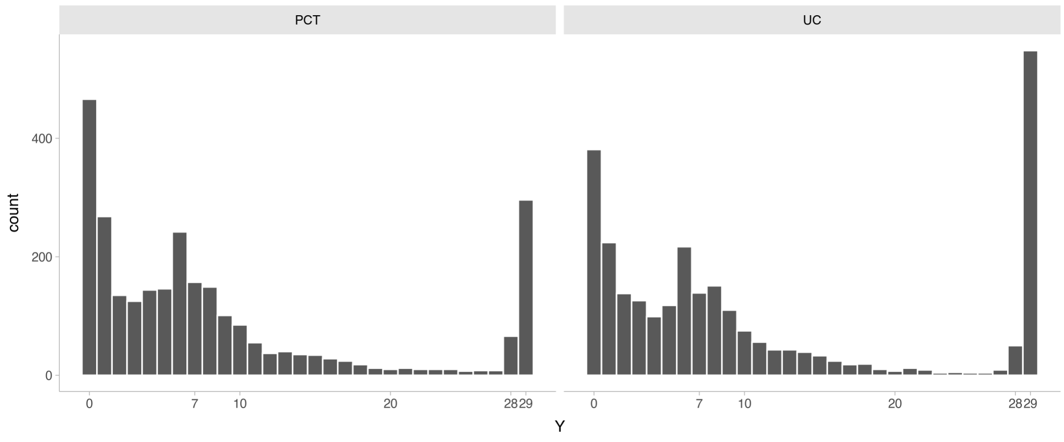
Imagine we have data from a RCT comparing two strategies (experimental = PCT and control = UC). These strategies aid physicians to decide whether a patient needs treatment with antibiotics or not. We then measure the number of days patients were treated with antibiotics for up until 28 days and if they were dead or not at the end of follow-up of 28 days.
When Y = 0 , the patient was alive at the end of follow-up and did not use antibiotics.
When 1 \ge Y \le 28, the patient was alive at the end of follow-up and Y represents the total duration of therapy in days.
When Y = 29, the patient died.
Thus, there are three different process happening and thus a single estimand won’t probably capture potential independent differences between treatments.
From this scenario, I could imagine at least these three questions:
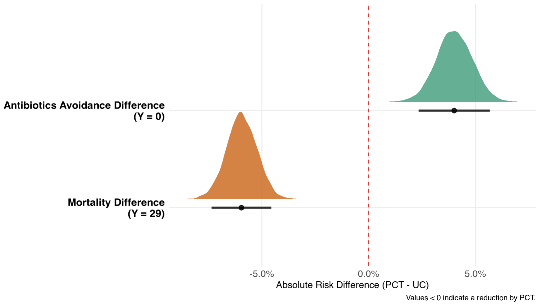
- Did the experimental strategy decrease the risk of getting treated with antibiotics?
- Did it decrease the risk of death?
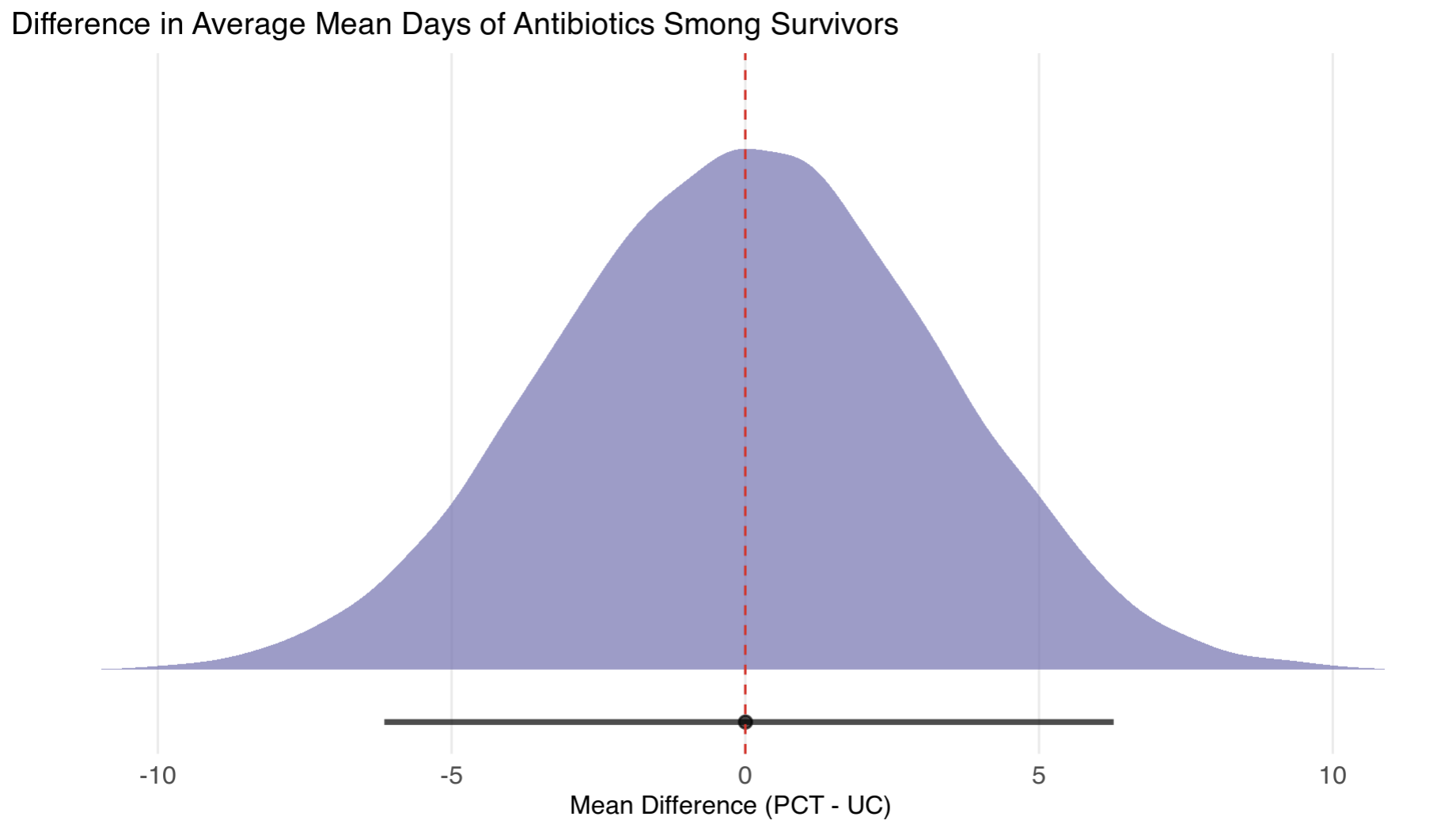
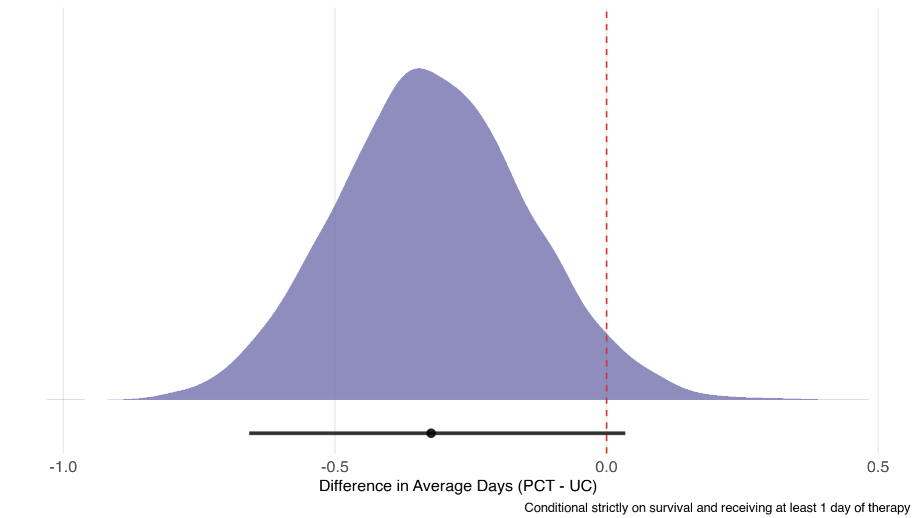
- In patient that did get treated with antibiotics and survived, did it reduce the total duration of therapy?
This example motivated me to fit a constrained partial proportional odds model to separely estimate treatment effect to answer these questions.
I simulated a dataset with 5453 patients (2715 in UC group) with ~0.2 in PCT and ~0.1 mortality rates in UC. Many patients didn’t get any antibiotics (Y=0) and many got around 7 days because this is a common duration for antibiotics.
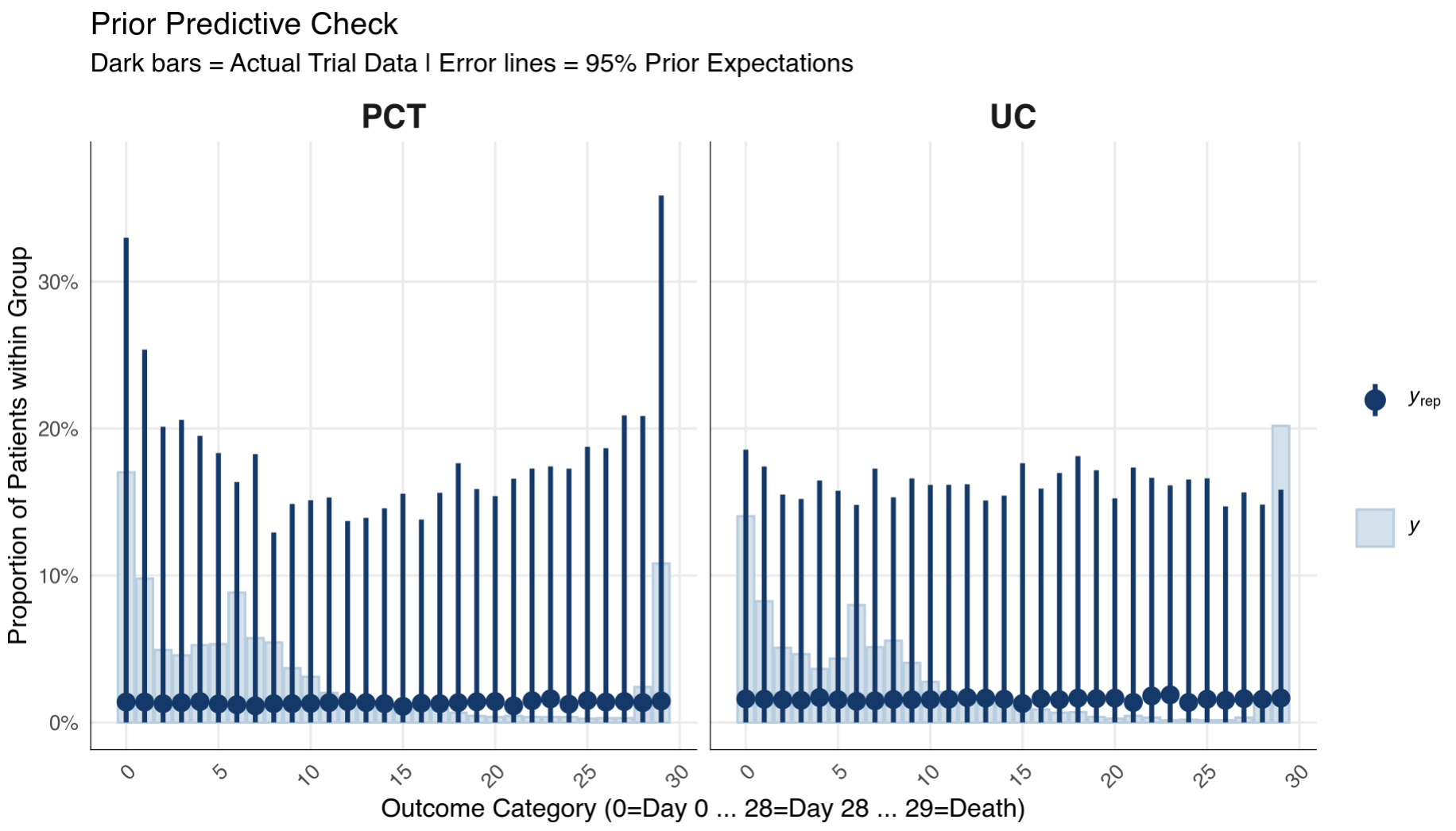
I then fitted a Bayesian model in Stan with weakly-informative priors for treatment effects and vague for intercepts:
Stan code
data {
int<lower=1> N;
int<lower=3> K;
array[N] int<lower=0, upper=K-1> Y;
vector[N] X;
vector<lower=0>[K] dirichlet_conc;
int<lower=0, upper=1> prior_only;
}
parameters {
simplex[K] pi;
real beta_duration;
real tau_avoidance;
real tau_death;
}
transformed parameters {
vector[K] cp = cumulative_sum(pi);
vector[K-1] alpha = logit(cp[1:(K-1)]);
vector[K-1] beta_c;
beta_c[1] = beta_duration + tau_avoidance;
for (c in 2:(K-2)) {
beta_c[c] = beta_duration;
}
beta_c[29] = beta_duration + tau_death;
}
model {
pi ~ dirichlet(dirichlet_conc);
beta_duration ~ normal(0, 0.82);
tau_avoidance ~ normal(0, 0.82);
tau_death ~ normal(0, 0.82);
if (!prior_only) {
for (n in 1:N) {
vector[K-1] mu = X[n] * beta_c;
int y_idx = Y[n] + 1;
if (y_idx == 1) {
target += log_inv_logit(alpha[1] - mu[1]);
} else if (y_idx == K) {
target += log1m_inv_logit(alpha[K-1] - mu[K-1]);
} else {
target += log_diff_exp(
log_inv_logit(alpha[y_idx] - mu[y_idx]),
log_inv_logit(alpha[y_idx-1] - mu[y_idx-1])
);
}
}
}
}
generated quantities {
array[N] int<lower=0, upper=K-1> Y_rep;
// ==========================================
// 1. POSTERIOR PREDICTIVE SIMULATIONS
// ==========================================
for (n in 1:N) {
vector[K] theta;
vector[K-1] mu = X[n] * beta_c;
theta[1] = inv_logit(alpha[1] - mu[1]);
for (k in 2:(K-1)) {
real raw_prob = inv_logit(alpha[k] - mu[k]) - inv_logit(alpha[k-1] - mu[k-1]);
theta[k] = raw_prob > 0 ? raw_prob : 1e-10;
}
real last_prob = 1 - inv_logit(alpha[K-1] - mu[K-1]);
theta[K] = last_prob > 0 ? last_prob : 1e-10;
theta = theta / sum(theta);
Y_rep[n] = categorical_rng(theta) - 1;
}
// ==========================================
// 2. CLINICAL ESTIMANDS (Exact Probabilities)
// ==========================================
vector[K] P_UC;
vector[K] P_PCT;
// Calculate P_UC (Baseline)
P_UC[1] = inv_logit(alpha[1]);
for (k in 2:(K-1)) {
real raw_prob = inv_logit(alpha[k]) - inv_logit(alpha[k-1]);
P_UC[k] = raw_prob > 0 ? raw_prob : 1e-10;
}
real last_prob_uc = 1 - inv_logit(alpha[K-1]);
P_UC[K] = last_prob_uc > 0 ? last_prob_uc : 1e-10;
P_UC = P_UC / sum(P_UC);
// Calculate P_PCT (Treated)
P_PCT[1] = inv_logit(alpha[1] - beta_c[1]);
for (k in 2:(K-1)) {
real raw_prob = inv_logit(alpha[k] - beta_c[k]) - inv_logit(alpha[k-1] - beta_c[k-1]);
P_PCT[k] = raw_prob > 0 ? raw_prob : 1e-10;
}
real last_prob_pct = 1 - inv_logit(alpha[K-1] - beta_c[K-1]);
P_PCT[K] = last_prob_pct > 0 ? last_prob_pct : 1e-10;
P_PCT = P_PCT / sum(P_PCT);
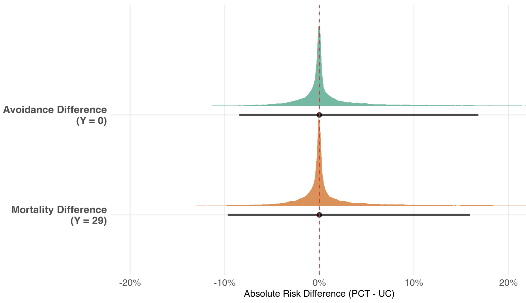
// --- Estimand A: Absolute Risk Differences (Boundaries) ---
real ARD_Avoidance = P_PCT[1] - P_UC[1];
real ARD_Mortality = P_PCT[K] - P_UC[K];
// --- Estimand B: Conditional Mean Days (1 <= Y <= 28) ---
real cond_sum_days_UC = 0;
real cond_prob_treated_UC = 0;
real cond_sum_days_PCT = 0;
real cond_prob_treated_PCT = 0;
for (k in 2:(K-1)) {
real day_val = k - 1;
cond_sum_days_UC += day_val * P_UC[k];
cond_prob_treated_UC += P_UC[k];
cond_sum_days_PCT += day_val * P_PCT[k];
cond_prob_treated_PCT += P_PCT[k];
}
real Cond_Mean_Days_UC = cond_sum_days_UC / cond_prob_treated_UC;
real Cond_Mean_Days_PCT = cond_sum_days_PCT / cond_prob_treated_PCT;
real Diff_Cond_Mean_Days = Cond_Mean_Days_PCT - Cond_Mean_Days_UC;
// --- Estimand C: Odds Ratios ---
real OR_Avoidance = exp(-(beta_duration + tau_avoidance));
real OR_Duration = exp(-beta_duration);
real OR_Survival = exp(-(beta_duration + tau_death));
}
Prior Predictive Checks:
Now for the actual model:
Diagnostics
All R-hats were really close to 1.0, N_eff/N were all above 0.8 and chains mixed well.
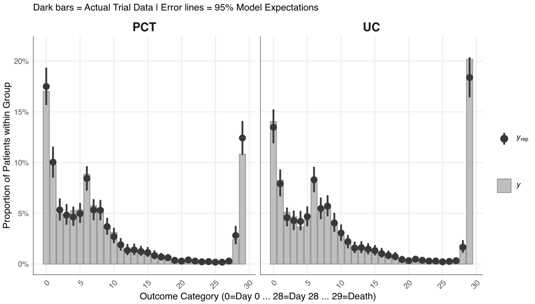
Posterior Predictive Check
Pretty good.
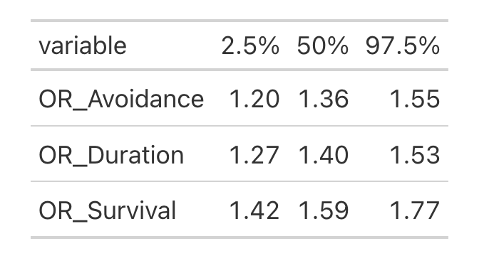
Results
And, of course, we can get odds ratios for each cutoff (Y = 0; Y = 29, and between):
Final remarks
I am no expert in Stan (closer to a newbie actually), thus I did use AI to help me write Stan code. My prior belief is that there ARE mistakes in the code, so please help me finding these and fixing it. Please! This is purely experimental.
Hope you enjoy it!
Full code: Bayesian partial PO · GitHub