I’ve decided to test the rmsb library on a cohort of women with breast cancer. Most authors have evaluated quality of life at the end of treatment by comparing median scores in women with or without intervention, usually using Wilcoxon tests. However, this method makes it impossible to predict what quality of life a woman may have in the future based on individual characteristics, such as age, the type of surgery (radical or breast conserving), etc… Here I have tried to predict the overall health status at 6 months, adjusted for various covariates.
A proportional odds model does not work because the assumption of PO for age and EORTC, both continuous variables, is not met. PPO models are excessively complex, and do not allow me to generate a nomogram. Therefore, the constrained CPPO model seems a good choice here.
The blrm function works nice, but the first problem I find is when using predict.blrm or summary.blrm, to represent the partial effects. This is the code and the error message it generates. I think all the variables are factors except age and EORTC.
> bs
Frequencies of Missing Values Due to Each Variable
       HE6        cir       linf    RR_PAC5   Esquema2   Estadio3 agespline1 agespline2     eopol1     eopol2
         0          0          0          0          0          0          0          0          2          2

Constrained Partial Proportional Odds Ordinal Logistic Model

 blrm(formula = HE6 ~ cir + linf + RR_PAC5 + Esquema2 + Estadio3 +
     agespline1 + agespline2 + eopol1 + eopol2, ppo = ~agespline1 +
     agespline2 + eopol1 + eopol2, cppo = function(y) y, data = DAT,
     file = "C:/Users/Alberto/Desktop/ bayes/mod_final.rds")


 Frequencies of Responses

    0  8.3 16.7   25 33.3 41.7   50 58.3 66.7   75 83.3 91.7  100
    5    1    4    1    9    2   43   18   35   20   48    8   23


                    Mixed Calibration/             Discrimination               Rank Discrim.
                Discrimination Indexes                    Indexes                     Indexes
    Obs217    LOO log L-457.59+/-12.05    g  1.135 [0.824, 1.386]    C   0.655 [0.634, 0.675]
 Draws4000      LOO IC   915.17+/-24.1    gp 0.225 [0.178, 0.263]    Dxy   0.31 [0.267, 0.35]
   Chains4     Effective p27.44+/-2.21    EV 0.173 [0.108, 0.228]
    p   11      B 0.212 [0.204, 0.221]    v   1.152 [0.518, 1.76]
                                          vp 0.041 [0.026, 0.054]

                   Mode Beta Mean Beta Median Beta S.E.   Lower   Upper   Pr(Beta>0) Symmetry
 cir=1             -0.6421   -0.6597   -0.6631     0.2635 -1.1533 -0.1314 0.0055     1.02
 linf=1             0.2645    0.2666    0.2639     0.3291 -0.3925  0.8805 0.7955     0.98
 RR_PAC5=1         -0.5593   -0.5886   -0.5851     0.3573 -1.3064  0.0788 0.0468     0.97
 RR_PAC5=2         -0.6983   -0.7197   -0.7206     0.3582 -1.4193 -0.0054 0.0232     1.00
 Esquema2=1         0.0086   -0.0048   -0.0018     0.2974 -0.5696  0.5804 0.4960     1.04
 Estadio3=1         0.0390    0.0310    0.0279     0.2968 -0.5660  0.6042 0.5382     0.97
 Estadio3=2        -0.4054   -0.4104   -0.4061     0.5216 -1.4637  0.6093 0.2082     1.01
 agespline1         0.0765    0.0781    0.0783     0.0286  0.0233  0.1337 0.9985     0.99
 agespline2        -0.1130   -0.1151   -0.1150     0.0369 -0.1904 -0.0474 0.0003     0.95
 eopol1             0.2334    0.2498    0.2490     0.0986  0.0621  0.4515 0.9955     1.02
 eopol2            -0.0013   -0.0014   -0.0014     0.0007 -0.0028 -0.0001 0.0200     0.99
 agespline1 x f(y) -0.0224   -0.0141   -0.0147     0.0210 -0.0556  0.0257 0.2455     1.06
 agespline2 x f(y)  0.0381    0.0230    0.0239     0.0280 -0.0351  0.0738 0.7962     0.92
 eopol1 x f(y)      0.0652    0.0808    0.0775     0.0565 -0.0222  0.1962 0.9375     1.16
 eopol2 x f(y)     -0.0003   -0.0004   -0.0004     0.0004 -0.0012  0.0004 0.1568     0.85

> Predict(bs)
Error in `$<-.data.frame`(`*tmp*`, "lower", value = c(-15.9968304854816,  :
  replacement has 2 rows, data has 3
> s <- summary(bs)
Error in xd %*% beta : argumentos no compatibles
>
Also I have problems with the nomogram…
> dd<-datadist(DAT)
> options(datadist='dd')
> bsix <- blrm(HE6  ~ cir * rcs(Age,3)+ linf+ RR_PAC5 + Esquema2+Estadio3  + pol(EORTC),
+             ~ rcs(Age,3)+ pol(EORTC), cppo=function(y) y, data=DAT, file='C:/Users/Alberto/Desktop/bayes/mod_finalint.rds')
> exprob <- ExProb (bsix)
>
> fun50<-function(x) exprob (x, y=50)
> fun65<-function(x) exprob (x, y=66.7)
> fun80<-function(x) exprob (x, y=80)
>
>
>
> M <- Mean (bsix)
> qu <-Quantile (bsix)
>
> med <- function (lp) qu(.5 , lp)
>
>
> nom.ord<- nomogram(bsix, fun=list(Mean=M, "Prob QoL>=50%"=fun50,
+                                      "Prob Qol >=65%"=fun65, "Prob QoL>=80%"=fun80), lp=F,
+                    fun.at=list(
+                      seq(20,90,10),
+
+                      seq(0.1,0.9,0.1),
+                      seq(0.1,0.9,0.1),
+                      seq(0.1,0.9,0.1),
+                      seq(0.1,0.9,0.1)
+                    )
+ )
Error in X %*% coefs[jj] : argumentos no compatibles
>
>
>
>
>
> plot(nom.ord)
Error in h(simpleError(msg, call)) :
  error in evaluating the argument 'x' in selecting a method for function 'plot': objeto 'nom.ord' no encontrado
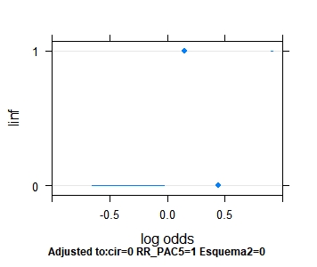
And with plot.predict with CIs out of range
You can edit earlier posts without adding multiple replies.
See https://hbiostat.org/fh/contacts.html for information about how to produce a minimal self-contained working example that I can use in debugging.
1 Like
Please put at https://github.com/harrelfe/rmsb/issues and let’s only deal with one issue at a time, resolving that issue before posting the next issue.
Ok, I also wanted to ask if it is the correct way to specify the CPPO model when the term that does not meet the PO assumption (Age) goes in an interaction cir * Age (cir is type of surgery, see code above). Also if the splines are well specified in the formula
I haven’t test that but I’m fairly certain that this should work:
blrm(y ~ x1 * x2 + x3, ~ x1 * x2, cppo=function(y) y >= 3)
The departure from PO should be applied to all main effect and interaction terms for x1 and x2.
1 Like
If the ordinal end point has many levels, an additional topic suggested but not specified in the 1990 paper is how to model non-linear relationships between coefficients for constrained terms. For example, how to code an upwardly concave parabola, or a downward or upward curve. Also what to do if there are outliers for some cut-off points that may influence the gamma parameter. Does it make sense to represent the coefficients of a multinomial model vs. the levels of the ordinal variable to make the regression diagnosis and decide the best fit?
The constraint can be of any shape you specify and will use whatever shapes you impose. If you need to estimate the shape of the constrain you’ll need things like monotone splines in Y interacting with covariates, which is not implemented in the function.
For example, here I fit a multinomial regression.
library(nnet)
test <- multinom(HE6  ~ cir * rcs(Age,3) +linf+ RR_PAC5 + Esquema2+Estadio3+ pol(EORTC), data=DAT)
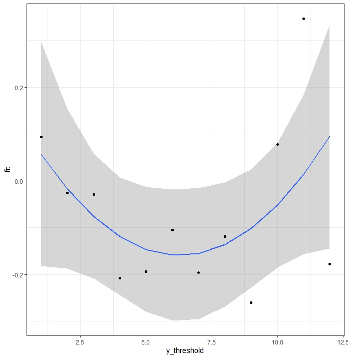
After that I have represented the coefficients of one of the variables against the cut-off points of Y.
coefi<-data.frame(coef(test)[,2:14])
coefi2<-gather(coefi, key = "variable",value = "coefficient",1:12)
coefi2$y_threshold<-rep(seq(1,12,1),12)
num<-coefi2$variable=="cir1.rcs.Age..3.Age"
coefi3<-subset (coefi2, num)

fit <- lm(coefficient ~  I(y_threshold) + I(y_threshold^2 ), data = coefi3)
summary(fit)
prd <- data.frame(y_threshold =1:12)
err <- predict(fit, newdata = prd, se.fit = TRUE)

prd$lci <- err$fit - 1.96 * err$se.fit
prd$fit <- err$fit
prd$uci <- err$fit + 1.96 * err$se.fit

ggplot(prd, aes(x = y_threshold, y = fit)) +
  theme_bw() +
  geom_line() +
  geom_smooth(aes(ymin = lci, ymax = uci), stat = "identity") +
  geom_point(data = coefi3, aes(x = y_threshold, y = coefficient))
A quadratic model is reasonable, and seems better than a linear model. How would this model be coded within the cppo function of the rmsb package?
If you really believed what the graph is estimating you could code cppo=function(y) abs(y - nadir of graph)
1 Like
Thank you very much, Professor Harrell, for your answer. I have already finished the article to predict the quality of life in women with breast cancer with the rmbs package, pending to polish these details and the code issue that doesn’t work. Regarding the cppo function, it is not very clear why a quadratic model Y= level * level^2 corresponds to cppo= function(y) abs (y - nadir y). Since this part is the key that distinguishes the Peterson-Harrell model from other options, I think it would be very useful for the rest of the users to clarify this point. For example, perhaps it could be better explained the code for monotonic increasing or decreasing functions, non-monotonic functions…, or even the way to use splines within cppo.
I was using absolute values because the graph looked more like that than quadratic to me. You could have used (y - y~ \text{nadi}r)^2, There are two partial proportional odds models in Peterson & Harrell (1990): the unconstrained one which is more flexible as you are implying you want to have, but takes many more parameters, and the constrained one which is a restricted one parameter per covariate version.
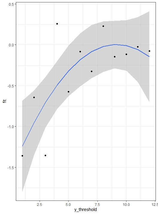
And for increasing functions such as 
Whether you use subjective visual checks or parameterized models, the degrees of freedom that you choose to give to a part of a model is part of the variance-bias tradeoff. This tradeoff is more tricky with smaller sample sizes because the width of credible intervals increases with more parameters and Bayesian power can be lost by not concentrating effects into fewer parameters. For the sample sizes we often encountered in human outcome studies (including clinical trials) the constrained partial PO model is a good compromise (in the above example perhaps with a linear constraint). You can think about it this way: many analysts don’t worry about the PO assumption and so they don’t fit exceptions to PO in their modeling. You are allowing for at least a first-order exception on the other hand.
1 Like
The Bayesian equivalent of the likelihood ratio test is very interesting in this constrained ordinal model. Since continuous variables deviate most from the PO assumption, it will often be necessary to evaluate the impact of interactions between a binary factor and splines. This is very important clinically, for example, to assess whether the effect of an intervention differs according to age, on a continuous basis.
I wanted to ask how to interpret a comparison of two models using compareBmods.
For example, here I have two models, the first one contemplates an interaction with a spline, the second one is an additive model. Can you please explain the interpretation of the result?
> bs_neuro3 <- blrm(HE6 ~ neuro2*rcs(Age,3) + stage + pol(EORTC), ~ neuro2*rcs(Age,3)+pol(EORTC),
                  cppo=function(y) , data=s)

> bs_neuro4 <- blrm(HE6 ~ neuro2+rcs(Age,3) + stage + pol(EORTC), ~ rcs(Age,3)+pol(EORTC),
                  cppo=function(y) , data=s)

> compareBmods(bs_neuro3,bs_neuro4)
Method: stacking
------
       weight
model1 0.175
model2 0.825
Not sure why you thought continuous variables would have more problem with PO.
The interpretation is best covered in McElreath’s book. I think of model 2 as being 0.825 likely to be the better of the two models in fitting the data generating process.
Thank you for the book recommendation. The book by McElreath seems very interesting to read in its entirety, not just for that particular topic. I don’t know why I assumed that for continuous predictors the violation of PO is more frequent. When splines are used, since the curve is more complex, it seemed to me that it would have to fail more times. Has this been simulated to see if this is the case?