I agree. But I can’t see the information for reanalysis…
It’s in Table 3, isn’t it?
I’ve taken Table 3 from the article:
https://www.nejm.org/doi/full/10.1056/NEJMoa2001282
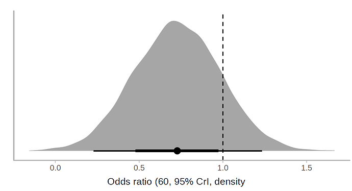
I applied a cumulative link model with the R brms package. According to this model, the use of lopinavir/ritonavir reduces the risk of outcomes or worse outcomes with odds ratio [OR] 0.72 (95% CrI, 0.43-1.20) under a non-informative prior. The posterior probability of obtaining an effect size >15% (OR<0.85) is 73%, which coincides with the Bayesian Cox model. Below is the halfeye plot:
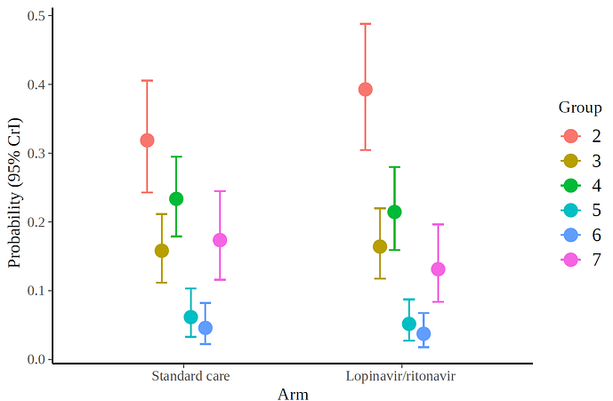
and the marginal effects according to the fitted model.
I also show the code:
lot<-data.frame(group=c( rep(2,43+28), rep(3,24+8),rep(4,20+25),rep(5,6+5), rep(6,5+3),rep(7,17+15)),
                treat=c(rep(1,43),rep(0,28),rep(1,8),rep(0,24),rep(1,25),rep(0,20),rep(1,5),rep(0,6),rep(1,3),rep(0,5),rep(1,15),rep(0,17)))

lot$group<-factor(lot$group, ordered = T)
table(lot$group,lot$treat)

library(brms)
fit3 <- brm(
  formula = group ~ 1 + treat,
  data = lot,
  family = cumulative("logit")
)
hypothesis(fit3, "treat1 < log(0.85)",alpha=.05)
marg<-marginal_effects(fit3, "treat", categorical = TRUE)The reanalysis here was referenced by Dahly et al. https://zenodo.org/record/3746512
That was @simongates touch.
For univariate proportional odds Bayesian models using Stan I am about to update the R rms package with a host of easy-to-use functions for plotting, estimation, credible intervals for indexes of predictive performance, nomograms, etc.
Cool, I see you’re active on many fronts. When will it be ready?
A few days. The trick is that I can make Linux and Windows packages for rms whenever I need them, but don’t know of an online Mac builder that lets me make a Mac executable package (I don’t use Mac).
 For frequentist models
 rms already has a lot of stuff for ordinal responses.
We were going to start an analysis to predict the quality of life of women with breast cancer according to the type of mastectomy. I better wait for that rms package update.
As a follow-up comment, NEJM finally accepted a letter based on this post, but in a very abbreviated format, without a figure. Furthermore, we could not explain the ordinal end point analysis, but several international authors expressed their views on the uncertainty of the study.
https://www.nejm.org/doi/pdf/10.1056/NEJMc2008043?listPDF=true
Wonderful, glad you submitted the letter. The response was unfortunately a non-answer. I cant help but feel that clinicians in general have a poor handle on bayesian probability & uncertainty. Something we need to work on.
The response was such a non-answer that I wrote to the author today to complain. The author missed the point that p-values had been completely misinterpreted. Hope to hear back. So glad to see @albertoca letter published. When will NEJM shore up peer review?
This is the best way forward. As the outcome was captured in an ordinal fashion, it makes sense to follow-up with a polr analysis. As a side note: given the urgency of the situation, why wouldn’t the authors make the original data (deidentified of course) available for further analysis?
They fixed the discrepancy between the HRs in the Abstract and Text (but no errata from NEJM). Turns out the HR 1.31 (0.95 to 1.85) was the “correct” HR.
Also, data for the ordinal outcome must exist for every day (otherwise they couldn’t work out time to improvement) so it would be really useful to see how the treatment effect varies over time, even just a visualisation of it without statistics.
Best way to model it seems to be incorporating time into an ordinal model as shown here http://hbiostat.org/proj/covid19/bayesplan.html. Gets my vote anyway!
This issue is quite pervasive, not only in NEJM. In Journal of Antimicrobial Chemotherapy I received the following peer review regarding the bayesian reanalysis:
Given the estimated size of the effect of lopinavir in the trial ‘Mortality at 28 days was similar in the lopinavir–ritonavir group and the standard-care group (19.2% vs. 25.0%; difference, −5.8 percentage points; 95% CI, −17.3 to 5.7)’, it is unfair to state as in the present submission ‘unless we were to consider that a 17% difference in survival is inconsequential’ given that the best estimate is 6% not 17%.
I am not convinced that we need a Bayesian re-analysis of the trial for considering that lopinavir should continue to be evaluated. The most obvious reason for that is the subgroup analysis regarding the delay between the beginning of symptoms to the inclusion in the study showing that if used in patients soon after the first symptom, the drug is likely to be beneficial, even though only shown in a subgroup analysis.
To conclude, I think the authors of the Cao et al NEJM paper have only reported their results in a transparent and honest manner that can be commended in a crisis period where many investigators are producing very poorly designed and reported studies that are none the less published even in high impact journals…
Thank you very much for this reply! I am trying to replicate the figures (and look at the Remdesvir study from the same group) but I am having trouble replicating the documentation of the survHE method, which I found here:
In particular, I can’t seem to figure out clearly how to include both arms in the matrices.
Best,
Alan
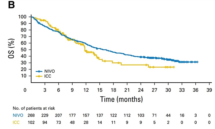
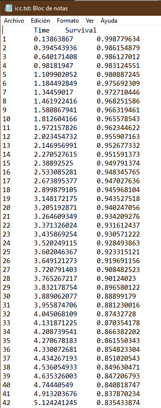
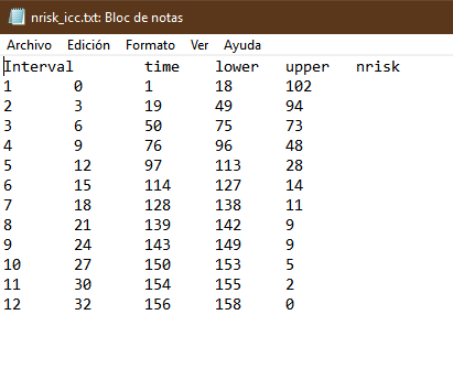
I’ll show you how it should look. In this example the trial had two arms. I show only one for simplicity. They are two files in txt format. What you may find hardest to understand is the table of numbers at risk. The key is that the third and fourth columns of the nrisk_icc file refer to the data within icc.txt, while the fifth column is the number at risk. Another issue is that you must make sure that survival always goes down, and time always flows forward. For each step generate at least three points. The most complex thing is the tails of the curve. It’s an art but the method works.
Hi Alan,
Perhaps I am a little late to the party but I have the solution for your specific question:
You must conduct the tutorial twice, one for each treatment arm. In the end, you should add a column in the “ipd_output” file generated by survHE::digitise to identify the respective treatment arm (remember that you should have two different files, one for each treatment arm). Finally, you put these two files together with something like dplyr::bind_rows().
Here is a code showing my workflow: Extracting data from KM curve (2 arms) · GitHub
Please note that you will not be able to directly replicate it (different data), but should be enough to help you.
