I have just started to read the paper. If those are the take-home messages, this is simply an awful approach IMHO, on bullet points 1, 2, and to a lesser extent 5. Here are some of the reasons I react this way:
- ANCOVA gains power and/or precision by explaining outcome heterogeneity by conditioning on pre-existing measurements that relate to Y. The resulting treatment effect is conditional, allowing comparisons of like with like. One should not do anything to uncondition (marginalize; average) the analysis but should make full use of the conditioning at every step.
- Fitting models separately by treatment group results in suboptimal estimates of residual variance, is highly inefficient statistically, and results in bias. Allowing for interactions with treatment in the primary analysis, if the primary analysis is frequentist, results in a huge power loss and in effect uses a weird prior distribution for heterogeneity of treatment effect.
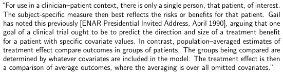
- Average treatment effect (ATE) should play no role whatsoever in a randomized clinical trial. The fundamental question answered by an RCT, which is even more clear in a crossover study but is also true in a parallel group design, is “what is the expected outcome were this patient given treatment A vs. were she given treatment B”. As I quote Mitch Gail in Chapter 13 of BBR:
- The recommendations fail to note a very simple fact. As John Tukey said you can make a great improvement in efficiency by just making up the covariate adjustment, getting the model completely wrong. His example was having clinical investigators make up out of thin air the regression coefficient for a baseline covariate. This will beat unadjusted analyses. Our enemy is inefficient unadjusted analysis and we don’t need to beat ourselves over the head worrying about model misspecification. The unadjusted analysis uses the most misspecified of all models.
Note: as shown in the Gail example in Chapter 13 of BBR, when there is a strong baseline covariate, say sex, the average treatment effect odds ratio is essentially comparing some of the males on treatment A with some of the females on treatment B. Not helpful.
To see the problem with ATE consider how this is usually improperly labeled PATE for population average effect, even though it is calculated from a sample with no reference to a population. For a sample averaged treatment effect to equal PATE, the sample would have to be a random draw from the population, or the analysis would have to incorporate sampling weights. RCTs do not use random sampling, and no one uses sampling weights in RCTs but instead (1) let the RCT sample stand on its own and (2) use proper conditioning as in ANCOVA.
An exceptionally important point for clinical trialists to understand is that, as Gail stated, an ATE that conditions on no covariates and does not use sampling weights will not estimate the correct population parameter in a nonlinear model. Conditional estimates, i.e., treatment effect estimates adjusted for covariates, are the ones that are transportable to patient populations having different covariate distributions than the distributions in the RCT. And if you should have conditioned on 5 apriori important covariates and only conditioned on 4, an odds or hazard ratio for treatment will be averaged over the 5th (omitted) covariate. But unadjusted treatment effects average over all 5 covariates, a much worse problem.
Here is an example to help in understanding the value and robustness of covariate adjustment in randomized experiments. Suppose the following:
- There are two treatments and the response variable Y is continuous
- There is one known-to-be-important baseline covariate X, and X is related to Y in a way that is linear in log(x): a rapid rising early phase, then greatly slowing down but never getting glad
- Ignoring X and having a linear model containing just the treatment term (equivalent to a two-sample t test) results in R^2=0.1
- Failing to realize that most relationships are nonlinear, the statistician adjusts for X by adding a simple linear term to the model, resulting in a model R^2=0.3
- The relative efficiency of the unadjusted analysis to the (oversimplified) adjusted analysis is the ratio of residual variances, which is \frac{0.7\sigma^2}{0.9\sigma^2} = 0.78, implying that an adjusted analysis on 0.78n subjects will achieve the same power as the unadjusted analysis on n subjects (here \sigma^2 is the unconditional var(Y))
- The false linearity assumption for X has resulted in underfitting, but ANCOVA is still substantially better than not adjusting for X; the unadjusted analysis has the most severe degree of underfitting
- Avoiding underfitting by adjusting for, say, a restricted cubic spline function in X, would result in an additional improvement. For example the R^2 may increase to 0.4, further lowering the residual variance, which decreases the standard error of the treatment parameter in the model and thus narrows the confidence interval and increases power.
Contrast this example with one where Y is binary and treatment effectiveness is summarized by an odds ratio when there is at least one important baseline covariate.
- The Pearson \chi^2 or less efficient Fisher’s “exact” test for comparing two proportions have a key assumption violated: the probability that Y=1 in a given treatment group is not constant. There is unexplained heterogeneity in Y that could be easily (at least partially) explained by X.
- The unadjusted analysis refuses to explain easily explainable outcome variation, and as a result the unadjusted treatment odds ratio tends to be closer to 1.0 than the adjusted subject-specific odds ratio.
- The standard error of the treatment log odds ratio may increase by adjusting for X, but the treatment point estimate will increase in absolute value more than the amount the standard error increases, resulted in an increase in power.
- Failure to correctly model a nonlinear effect of X will result in a suboptimal analysis that is still superior to the unadjusted analysis, which has the worst goodness of fit (because of it having the most severe underfitting).
- An adjusted analysis more closely approximates a correct answer to the question “Were this subject given treatment B what do we expect to happen as compared to were she given treatment A?” The unadjusted odds ratio is a sample averaged odds ratio that only answers a question about a mixed batch of subjects. Its interpretation essential relates to asking how some subjects on treatment B with lower values of X compare to some subjects on treatment A with higher values of X. Anyone interested in precision medicine should refuse to compute unadjusted estimates.
On a separate note, it is important to realize that covariate adjustment in randomized trials has nothing to do with baseline imbalance.
Resources
- Commentary on Improving Precision and Power in Randomized Trials for COVID-19 Treatments Using Covariate Adjustment, for Binary, Ordinal, and Time-to-Event Outcomes by Frank Harrell and Stephen Senn
- The Well Adjusted Statistician by Stephen Senn
- Analysis of Covariance in Randomized Studies by Frank Harrell
- Statistical Issues in Drug Development by Stephen Senn
- Should We Ignore Covariate Imbalance
- Comments on FDA guidance draft by Jonathan Bartlett