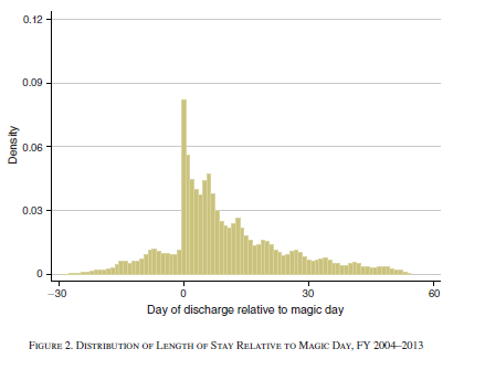
I am doing a study on manipulated hospital discharges using a similar methodology as this paper: https://pubs.aeaweb.org/doi/pdfplus/10.1257/aer.20170092. In short, we observe that patients are more likely to be discharged directly after a higher tariff rate has been reached, leading to distribution of discharges such as this:

- I estimate the following probit model:
glm(close ~ time + time^2 + t_at + t_before , family = binomial(link = "probit"), data = mydata)
Where time is the duration of the treatment and the dummies are at the t=0 where the tariff changes and at t=-1, directly before the tariff changes.
- Next I calculate the probability of a discharge at t=0 and at t=-1 and calculate the hazard-ratio by dividing those two. This would indicate the speed at which the probability of discharge changes between those two times.
Instead of the steps in 2., the referees of my paper would rather see average marginal effects at t=0 and t=-1.
Question: If I calculate average marginal effects, can I still calculate their ratios and call that a hazard-ratio? I assume not. But how can I indicate the rate of change between the two times?
Note1: I do something similar to Table 4. in Eliason. I compare different subgroups to test whether certain patient characteristics affect the extent of discharge manipulation. The referee says that hazard-ratio is economically difficult to interpret and instead I should add interaction-terms to my probit model and calculate marginal effects for those. But the “rate of change” effect so nicely captured by Eliason is lost. Or is it not?
Note2: For example, when testing whether women are more likely to be manipulated I would run : glm(close ~ time + time^2 + t_at + t_b4 + t_at*female + t_b4*female , family = binomial(link = "probit"), data = mydata)
1 Like
What is it that the referee is asking you to uncondition upon / marginalize over?
Instead of thinking of this as a “make estimates at two time points” problem why not think of it as “model time flexibly problem”? Usually flexible modeling implies flexible smooth curves but in your case it makes sense to not impose a continuity restriction on the model with respect to time. As an aside you can allow for approximate discontinuities by putting knots in a cubic spline function very close together.
A binary logistic model (or probit, if you really insist) can have in it time since admission (optimally in hours but at least in days) modeled as g(t - t_{0}) plus patient characteristics, where t_{0} is the magic day for the patient. A second time function h(t) models absolute time (hours or days from admission). h(t) would be smooth, e.g. a restricted cubic spline function. g(t) could have a discontinuity at zero. In simplest form g(t) = [t \geq 0] where [c]=1 if c occurs, 0 otherwise. If you wanted to use a linear spline with zero order continuity and first order discontinuity (discontinuity in slope) you would use g(t) = \beta_{1}t + \beta_{2}t_{+} where t_+ is t[t > 0] which equals \max(t, 0). To model a linear effect with zero order discontinuity (bilinear regression) use g(t) = \beta_{1}t + \beta_{2}[t > 0] + \beta_{3}t[t>0]. This latter one is a good starting point then you can extend that to allow for nonlinearity on both sizes of zero by adding appropriate quadratic and cubic terms.
Once you have the model, which needs to handle non-discharged patients also (a state transition logistic model would do this, to account for deaths), you can pick a few covariate settings (e.g., age and sex combinations) and compute the estimated discharge probabilities as a function of time. You can pick off example points from these curves and look at their absolute probabilities (at say t=-1 vs. t=0 vs. t=1). You could also draw 6 time curves for 2 sexes \times 3 ages.
Your original model has zero order discontinuities in it (which is appropriate) but assumes flat relationships on either side of the magic day, which is not consistent with the histogram.
 It strikes me for this particular problem that modeling accumulative cost as a time dependent variable, without using the magic time, may be a more direct solution.
1 Like

 It strikes me for this particular problem that modeling accumulative cost as a time dependent variable, without using the magic time, may be a more direct solution.