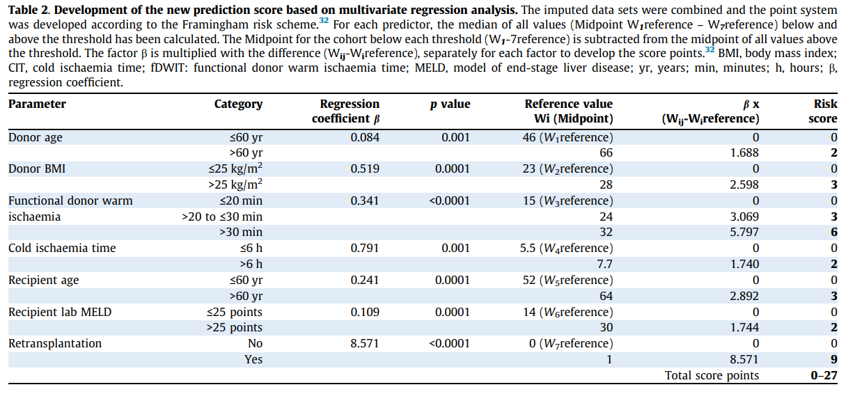
I’ve run out of ideas for the regression table below, which is from a prediction model for liver transplantation. The paper is available here. The primary outcome was graft failure at 1-year, and the authors fitted a logistic model. So far, so good. Here are the results.
Looking at the first two columns, it appears that all the continuous variables have been dichotomized except the last one, which was not continuous. The next column is the coefficients \beta. As this is a logistic model, it must either be a log odd ratio or an odds ratio. Unfortunately, all signs are positive, which leaves us in the dark. Using common sense, maybe the OR is reported because exp(8.57) would be insane? It seems that for one of the variables with three categories, one coefficient was not reported. Also, one coefficient seems to be on the wrong line; no way Retransplantation=NO is associated with a higher risk. The whole paper’s point is that retransplantation is a big no-no (using a DCD liver). The other coefficients make more sense (e.g., younger donors, smaller BMI, shorter ischemia time all reduce the chances of graft failure).
However, in the next step, the authors derived a risk score system. For example, with Donor age and using a cuffoff of 60 years, they calculated the median for the younger and older group (46 and 66); they call them midpoints. The difference is 20 years, so they multiply the difference in the medians with the coefficient 20 \times 0.084 = 1.68. Thus, the \beta X is basically the effect when going from 46 to 66 years, and the Risk score is just the rounded version of this.
Given this procedure, I would expect that they did not dichotomize before fitting the regression model but subsequently for the midpoints. This would also explain that there is only one coefficient for functional donor warm ischemia time. But I would also assume that they did this step on the log OR scale; that would make more sense, wouldn’t it? Thus, I conclude:
They did not dichotomize to fit the logistic model. All variables were entered into the model as continuous data, and the last was binary. Thus, you get one coefficient per variable. However, they did not report the intercept.
The \beta are log ORs due to the way they constructed the risk score.
Yes, the 8.571 is insane, reflecting a more than 5,000-fold increase in the chance of graft failure. I would love to see the uncertainty around this effect, but the authors failed to report standard errors or a 95% confidence interval. If the problem is complete separation, I would expect the p-value to be very high, not very small.
The Table is terrible, or maybe it is me who is very, very confused.
I would be very grateful for tips and advice and whether I am on the right track. I am not a Sherlock Holmes.
Please edit your post to provide the full citation for the paper from which the table was extracted.
I think that the authors did indeed report odds ratios, and that they committed a blunder of the first order by adding them rather than adding log OR. This will make helpful patient characteristics turn out to be harmful in the score. This has been written about by @Ewout_Steyerberg@ESteyerberg and myself in letters to the editor. NEVER add ratios.
It is extremely important to determine whether the dichotomization occured before vs after fitting. If it occured before fitting then all of the variable effects are misleading because they did noit properly condition on full covariate information, and this makes more variables appear to be prognostic.
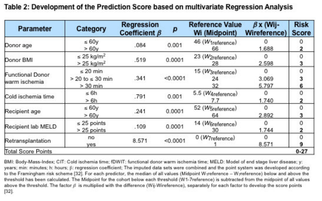
Thank you very much for the response. I researched more to find out whether the data was continuous or dichotomous to fit the model and found an approved manuscript version, which was still in the author’s original formatting. The table looks as follows:
Here, the effect estimates were vertically centered compared to the published version, where they were aligned with a specific level of the categorical variable (Table 2 in my initial post above). This may indicate that the data was not dichotomized before fitting the model, and we see one coefficient for functional donor warm ischemia time, which would require two coefficients if it had been dichotomized. I conclude with caution the data was not dichotomized. That is good news.
Now, if we assume continuous data, I would say the 0.084 is a log OR and not an OR, thus exp(0.084) = 1.08. It is more reasonable that there was an 8% increase in the chance of graft failure for each additional year increase in donor age. On the other hand, if 0.084 was an OR, then each additional year in donor age would result in a 92% reduction in the risk of graft failure. That is not plausible. Thus, I conclude the effects were log OR. That is also good news, so the author did not make the major blunder of adding up ratios in the construction of the risk score.
However, this still leaves us with the log OR of 8.571 for retransplantation, corresponding to an OR of exp(8.571) = 5,276. It might be explained when almost all the retransplantations resulted in graft failure. It is most likely what happened.
So, I hope this makes sense and is the most plausible scenario? Then, it may not be as bad as it appeared at first.
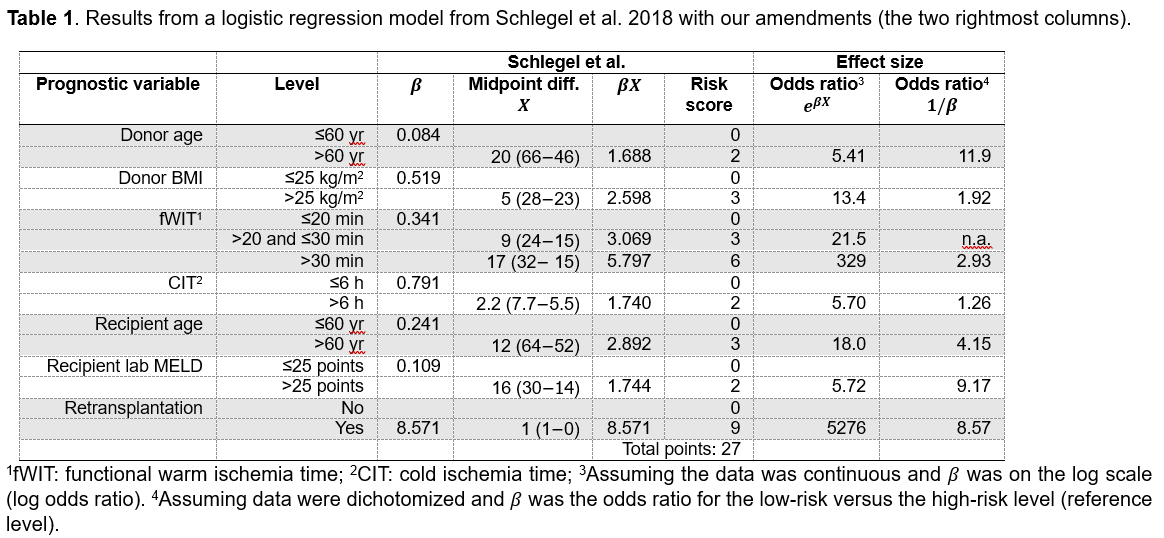
Okey, I have an update on this matter. I concluded in my last post that “it may not be as bad as it appeared at first.” Meanwhile, I have changed my mind. I think it is most plausible the coefficients reported as \beta were indeed odds ratios (and not log odds ratios). That is also what Frank said in his post. I don’t believe in odds ratios of 5276 or 329. Assuming data were dichotomized and \beta was indeed the odds ratio for the low-risk versus the high-risk level (reference level), we get more plausible results. I give a nice overview in the Table below. If this is true, the risk score is compromised, i.e., higher donor age and higher recipient MELD is a higher risk than a retransplant or longer warm ischemia time; in other words, the weights assigned by the score points are not correct.
I have written a letter to the editors of the Journal of Hepatology. The letter was rejected with the reason, quote, “it doesn’t appear to be an issue of ethics you are raising, rather methodologic skills”.