In linear regression, most of the methods that combat the two common problems of heteroskedasticity and non-normality are designed to counter the effect of one-problem only (either hetero or non-normality; not both in the same time).
One of the rare methods that combat both problems is one type of wild bootstrapping (it has an R-package for that).
On my searches for solution of the two problems, I found an R-package designed to do White-test (for heteroskedasticity) but conducted via bootstrapping (I guess package name is “whitestrap”). In many times when I try this package to obtain a bootstrap test of heteroskedasticity, I found good results (the bootstrap p-value of white test is generally larger than the conventional White test; this is under replications = 2000 or 1000). Once I increase the replications (B = 5000), the P-value goes towards non-significance, and usually once you try B = 10,000, non-signifiance is surely obtained (which is what we hope).
After such experiments on bootstrap white test, can one say that doing a bootstrap regression (of a model contaminated with both non-normality and hetero) with high replications (say 10000) would solve both problems, non-normality and hetero?
I’m not sold on that overall approach for several reasons.
- The Huber-White robust covariance matrix can give you the right answer to the wrong question. It can’t fix having less meaningful parameters due to model misspecification especially getting the transformation wrong.
- Even in simple situations it is not clear how Y should be transformed before doing parametric modeling.
- In general the bootstrap tells you how bad something is but not how to fix it.
- Semiparametric ordinal regression models cut through much of this:
- They are Y-transformation invariant
- The are completely robust to Y-outliers
- The can provide all needed readouts, including effect ratios, cumulative probabilities, individual cell probabilities, quantiles, and the mean
- They handle lower and upper limits of detection, floor and ceiling effects, bimodal distributions, heteroscedasticy (to some extent), excessive ties anyone in the range of Y
A resource for semiparametic models is here and here is a detailed case study of ordinary regression for continuous Y. It uses the R rms packge orm function which can handle more than 6,000 distinct Y values, i.e., it can do calculations efficiently with > 6000 intercepts in the model. A Bayesian counterpart to this is here.
Dear Professor @f2harrell,
What do you mean by the sentence above: “In general the bootstrap tells you how bad something is”?
I have a few questions about the bootstrap methods from the rms package (using bootcov() and Predict()).
On pages 200-201 from the RMS book you have the following:
b ← bootcov(f, B =1000)
Then,
- Predict(b, x, usebootcoef = F) ------------------ “Boot covariance + Wald”
- Predict(b, x) ----------------------------------------- “Boot percentile”
- Predict(b, x, boot.type = 'bca ') ----------------- “Boot BCa”
- Predict(b, x, boot.type = 'basic ') --------------- “Boot basic”
- Predict(b, x, conf.type = ‘simultaneous’) ----- “Simultaneous”
If I specify bootcov(f, B =1000, coef.reps = T), then I can use these coefs to obtain “Boot percentile”, “Boot BCa” and/or “Boot basic” 95% CIs later on, using the Predict() codes above, correct?
Or, I can specify Predict(b, x, usebootcoef = F) to obtain “Boot covariance + Wald” 95% CIs. These CIs do not rely on the bootstraped coefs, and are calculated using standard formula and a robust covariance matrix, which is estimated by means of resampling, is that right? In that case, would this be somewhat equivalent to using robcov(), which also returns a robust covariance matrix?
It seems that the focus in the RMS book is on using the bootstrap for model validation:
“In this text we use the bootstrap primarily for computing statistical estimates that are much different from standard errors and confidence intervals, namely, estimates of model performance” (RMS, p. 109).
But what are the main purposes of using these different types of CIs (including the “Simultaneous” one) within the context of inference?
For instance, I used the code above (RMS book, p. 200-201) on my own data/analysis and obtained the following (see image attached, which is inspired by Fig. 9.5 (RMS book, p. 204)).
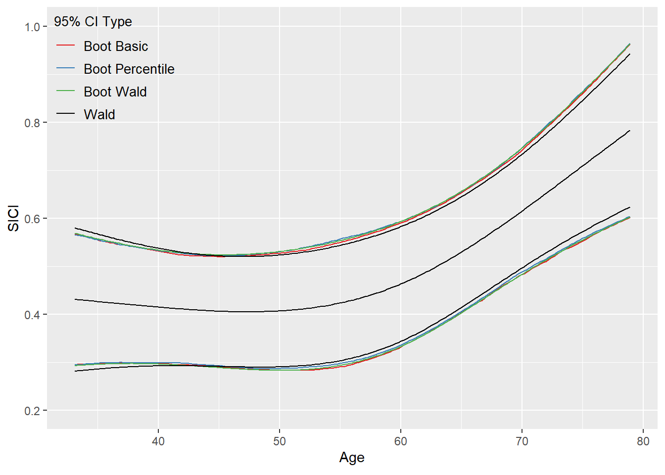
My main goal is to test the association between Age and SICI (the 2df test from the anova() is highly significant).
This is my model. Let’s assume for now that it is correctly specified:
ols(SICI ∼ rcs(Age, 3) + rcs(FM, 3) + rcs(Time, 3) + Sex + Side + Type)
Turning back to your sentence at the top… What are these different confidence bands telling?
Apologies for the long message.
Thank you for your attention!
Your perceptions are correct. And yes RMS uses the bootstrap more for model validation than for confidence intervals. There are so many bootstraps for the latter because they have different performance (e.g., accuracy of confidence interval coverage probabilities). The bootstrap that seems to work best for confidence intervals is the studentized bootstrap t but it is harder to implement (which is why you don’t see it in my text).
Formatting note: enclose code in single back tick marks instead of italics markup.
Thank you.
But why would one use the bootcov() for inference? For instance, in my case (association between Age & SICI), what would be the purpose? Can I think of it as a safeguard measure against deviations from model assumptions (e.g., non-normality and/or non-constant variance of residuals)? A way of obtaining trustworthy/reliable estimates/CIs?
Also, besides using it for obtaining CIs (e.g., through summary(), contrast(), and/or Predict()), what’s the idea behind passing the bootstraped model through the anova()? For instance, b <- bootcov(f); anova(b).
Sometimes the bootstrap covariance matrix is more accurate than the traditional information matrix-based one, especially if the model is misspecified. But I’ve seen a case with imbalanced logistic regression where all bootstrap methods worked worse than using the information matrix.
Ok, thank you.
Apologies for being so insistent about this, but I’m replying to a reviewer and just want to get my head around these concepts.
Is it correct to say that we can use bootstrap (in my case, bootcov()) to get robust estimates of association (anova(bootcov())) and robust predictions/partial effects plots (ggplot(Predict(bootcov()))) in ols()?
By robust I mean that the multiple df tests from anova() and the CIs from Predict() are not affected by deviations from the model assumptions of normality of the residuals & constant variance of the residuals when bootstrap is used.
For instance, in the rms manual, we have the following:
“When the first argument to Predict is a fit object created by bootcov with coef.reps=TRUE, confidence limits come from the stored matrix of bootstrap repetitions of coefficients, using bootstrap percentile nonparametric confidence limits, basic bootstrap, or BCa limits. Such confidence intervals do not make distributional assumptions.”
By distributional assumptions, do you mean the assumptions of normality of the residuals & constant variance of the residuals?
Yes to the last question. But to the earlier question we are using the bootstrap to estimate standard errors by using it to estimate the whole variance-covariance matrix without assuming correctness of the model, but this is not to get robust estimates of association. We are still using maximum likelihood for that.
Recalling that the bootstrap is an approximate method, and that there can be difficulties in choosing which bootstrap variant to use, a better strategy is to use more versatile models. There are multiple ways to do that, including semiparametric models and Bayesian parametric models that include parameters that relax model assumptions, puttin priors that allow model assumptions to be true but as the sample size increases more flexibility is allowed. This strategy is more likely to provide highly accurate uncertainty intervals.
Thank you very much, Professor.
So it seems that there is no need to pass the bootstraped model through the anova (e.g., anova(bootcov())) in order to test for associations between predictors and the response. Is that correct? Aren’t these tests of association from rms::anova() affected by deviations from distributional assumptions?
If that’s the case, then in the context of inference, bootcov() would be used only to produce robust CIs through summary(), contrast(), and Predict(), if I understood correctly.
Not necessarily; yes; not necessarily
Sorry, not sure I’m following…
Model: ols(y ~ rcs(x1, 3) + rcs(x2, 3) ...)
The residuals look somewhat heteroskedastic so I’m using robcov() and bootcov() for obtaining more accurate CIs through Predict() and contrast().
The multiple df tests of association from anova(fit), anova(robcov(fit)), and anova(bootcov(fit)) are all concordant in terms of significance, but the p-values change slightly.
I understand that anova(), Predict(), and contrast() are complementary. For example, as you already mentioned, when the multiple df tests of association from anova() are significant, this gives us more license to interpret partial effects plots (ggplot(Predict(fit))).
But what’s the purpose of doing anova(robcov(fit)) and anova(bootcov(fit))? Do they have a place when we have deviations from distributional assumptions (e.g., heteroskedastic residuals)?
Thank you.
They have different properties and you can’t always decide which one is better. I tend to use robcov more often. But the way you’re thinking about the problem is a bit too much divorced from goodness of fit assessment. Getting the right standard errors of the wrong quantities may not help.
Hi Professor, thank you for your feedback.
I don’t think I understand this: “But the way you’re thinking about the problem is a bit too much divorced from goodness of fit assessment. Getting the right standard errors of the wrong quantities may not help.”
My goal is to test the associaton of a brain activity marker (SICI, continuous variable) with a clinical test of disease severity (FM, integer values, ranging from 5 to 66) in stroke patients. I also have other variables at hand, such as Age, Sex, Time since stroke, Side and Type of stroke. I decided that it would make sense to test the association between FM and SICI by using ols(), with all the other variables as adjustment variables. I also decided to relax the linearity assumption by transforming the continuous predictors (Age, Time, and FM) with rcs(), using 3 knots:
ols(SICI ~ rcs(FM, 3) + rcs(Age, 3) + rcs(Time, 3) + Sex + Side + Type)
I’m taking this as a pre-specified model.
From the anova() output, it is interesting that FM, Age, and Side (but not the other predictors) seem to be associated with SICI, and that the only predictors that seem to be important for controlling for are Age and Side, as when these are dropped from the model, the association between FM and SICI disappears. Nevertheless, I decided to keep all the variables in the model, as pre-specified.
As you illustrate on Section 1.6 of RMS (Regression Modeling Strategies - 1 Introduction), empirical model selection through gof checking tends to lead to distorded statistical inference. On the other hand, using a pre-specified flexible model tends to lead to more acurate inference, as here the fit would be assumed to be adequate and there would be less model uncertainty.
Also, regarding your recommendations on Section 1.6.1 of RMS (Regression Modeling Strategies - 1 Introduction):
"Rather than accepting or not accepting a proposed model on the basis of a GOF assessment, embed the proposed model inside a more general model that relaxes the assumptions, and use AIC or a formal test to decide between the two. Comparing only two pre-specified models will result in minimal model uncertainty.
- More general model could include nonlinear terms and interactions
- It could also relax distributional assumptions, as done with the non-normality parameter in the Bayesian t-test
- Often the sample size is not large enough to allow model assumptions to be relaxed without overfitting; AIC assesses whether additional complexities are “good for the money”. If a more complex model results in worse predictions due to overfitting, it is doubtful that such a model should be used for inference."
1) What could be a more general model than my current one? A model with interaction terms or perhaps a semiparametric model?
2) What I don’t understand is that if I pre-specify 2 models (as per above), then select the best one (using e.g., AIC), does that mean I don’t need to worry about gof checks for this model (e.g., inspection of residuals) and simply stick with it?
3) From your sentences at the top of my message, I take that you are implying that my model is incorrect because I have heteroskedastic residuals. I think this is what is confusing me. It sounds as if the take home message from this was: “If your residuals look bad then there is no point in using robcov() or bootcov() for your inferences as your model is probably wrong.”
Mainly, a semiparametric model. But I don’t think you can compare AIC between a parametric model and a semiparametric one. On 3) largely yes. For example if you should have taken log(Y) but didn’t, residuals will look bad, a the sandwich estimator will just cover that up and give you better standard errors on completely wrong parameters.
Does orm accommodate repeated measures? Otherwise do you have another suggestion for dealing with heteroskedasticity and non-normality of residuals in the context of repeated measures? I already tried a few transformations, including log(Y), sqrt(Y), and (1/Y), but none of these helped enough.
I considered bootstrapping the fixed effects of a mixed model.
In the frequentist domain, the rms package orm function and the VGAM package vglm functions will fit ordinal Markov models. For Bayesian models see the rmsb and brms packages, which also allow for random effects. Markov models tend to fit better than random effects models for serial data; see this. I prefer Markov models because they are so general, applying easily to binary, ordinal, nominal, continuous, and censored Y.
Do they also apply if Y is a proportion?
Is Y a proportion in its most primative form, i.e., is not a summary statistic from a series of binary observations that could have been analyzed as separate units?
I have two scenarios in mind:
- Repeated measurements of hematocrit in kidney transplant patients
- Repeated measurements of the percentage of time that the concentration of an antibiotic remains above the minimum inhibitory concentration ( time above MIC)
Part 1 looks straightforward. For part 2, it is generally not a good idea to coursen the data before analysis but instead to analyze the rawest form of the data then compute quantities of interest from a function of the (efficiently) estimated parameters. That way there is credit for close calls, and no artifacts are introduced because of boundary issues. For example if you had the concentration of an antibiotic measured hourly for 24 hours, you could compute the expected time above MIC. With a Markov multistate semiparametric model this is just a sum of state occupancy probabilities where the state denotes being above MIC.