How do I analyse the functional form of the relationship between a covariate to the hazard ratio in a Cox proportional hazard model?

Hi there,

I’m analysing the functional form of a continuous covariate to the hazard ratio in a Cox proportional hazard model. I’d like to compare a linear model to a model where the covariate is log transformed. I have two specific questions:

  • What is the appropriate method for visual inspection?
  • Apart from visual inspection, should I do a formal test to compare the two models?

Fe, this paper (link to paper) used martingale residuals for visual inspection, and a partial likelihood ratio test to compare a model with linear terms and a model using fractional polynomials.

Kind regards,
Linda

1 Like

it would surely be covered in Frank Harrell’s book but i don’t have it to hand. I know i have seen in practice people simply add quadratic or cubic terms and look at the change in -2logL or akaike’ information (aic). The only reason for doing a formal test i guess is if you must pre-specify in an analysis plan, then you can state clearly what the criterion will be

I’ll just add that often a log transformation does not fit well enough, which is why it’s usually better to fit a flexible function such as a restricted cubic spline function and be done with it. Testing for “significance” of the added nonlinear terms leads to temptation, i.e., removing the terms, which can ruin p-values and confidence limits. Plot the fitted curve to interpret it.

1 Like

Piggybacking on this question.

I am interested in visually inspecting whether a variable is linearly associated with survival in a time to event model. Based on my understanding, fitting a naïve model without any transformation of a continuous variable, the hazard ratio will be an estimate of the effect on the hazard when increasing the variable by one unit. If the variable is log2-transformed, the hazard ratio will be an estimate of the effect when doubling the variable.

Both these analyses should assume (1) proportional hazards over time as well as (2) that the hazard rate is proportional over varying levels of the variable. It is the second point I’m interested in here, i.e. whether I can assume that the effect (on the hazard rate) of “increasing” my (untransformed) variable of interest from 10 to 20 is similar to increasing it from 20 to 30. For a log2-transformed variable, if I understood correctly, one would be interested in whether an increase from 10 to 20 would be similar to increasing it from 20 to 40.

I am trying to use real data to explore functional forms, but struggle to find out whether I got the code right (see below) to plot the hazard rate vs a continuous variable (univariable model).

# Histogram of the marker’s distribution
p1 <- df %>%
    ggplot(aes(x = marker))+
    geom_histogram(bins = 50)+
    theme_dca()+
    labs(title = "Histogram of marker values, N=270")
# Untransformed
fit <- cph(Surv(time, endpoint) ~ marker, df)
p2 <- ggplot(Predict(fit, marker = seq(min(df$marker), max(df$marker), length = 200))) +
    #scale_x_continuous(limits = c(0, 300))+
    labs(title = "Untransformed")
 # Log2-transformed   
fit <- cph(Surv(time, endpoint) ~ log2(marker), df)
p3 <- ggplot(Predict(fit, marker = seq(min(df$marker), max(df$marker), length = 200))) +
    scale_x_continuous(limits = c(0, 300))+
    labs(title = "Log2")
fit <- cph(Surv(time, endpoint) ~ rcs(marker,4 ), df)
p4 <- ggplot(Predict(fit, marker = seq(min(df$marker), max(df$marker), length = 200))) +
    scale_x_continuous(limits = c(0, 300))+
    labs(title = "RCS 4 knots")

Output from the code above

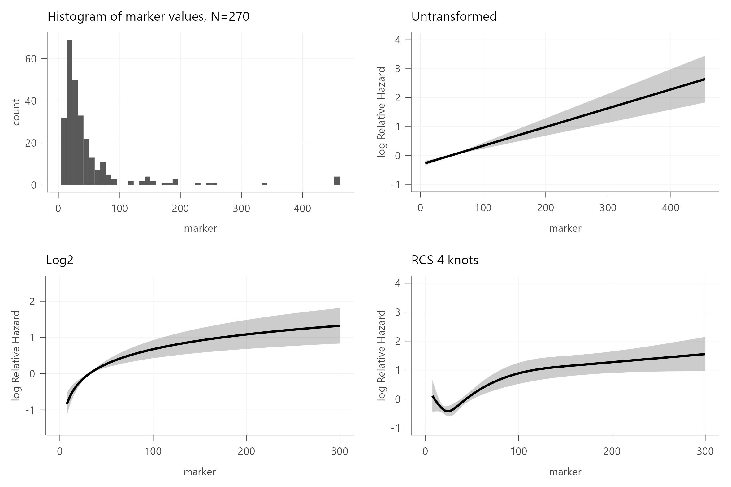
I understand from Harrell’s post above that fitting flexible functions like rcs() is useful – but (given that my code above is correct) I am not entirely sure how to move forward. I think both the log2 and rcs-transformed data indicate a departure from linearity, particularly at low concentrations. (Since this is a circulating analyte this is hardly surprising.) But does this mean that the hazard ratio from my log2 model cannot be directly interpreted? The RCS model also suggests departure from linearity, but as far as I’ve understood this transformation is flexible enough to handle non-linear relationships – so what would be the natural next step in my case? And I suppose the interpretation would be conditional on (omitted) covariates that may confound or interact with the variable?

I’m not a fan of the philosophy of trying different things and seeing what works best. Rather I recommend pre-specifying a model in consultation with subject-matter experts. As discussed here when the subject matter expertise is not available, fit a function that is as flexible (has as many parameters) as the effective sample size (here, the number of events) will allow, and be done with it.

1 Like

Thanks for the quick reply!

My question actually arose due to a question from a colleague about using change in the particular marker as a surrogate, biochemical endpoint for a clinical study. (This is far from my field of expertise - I’m a molecular biologist albeit with a great interest in statistics.)

More specifically, they wanted to know whether a 30% reduction in the marker would be a reasonable endpoint. Across several cohorts, the marker (log2-transformed) is associated with a relevant clinical endpoint,

While I’ve already suggested that they should consult a biostatistician with expertise on this field, they want some information to help guide them in formulating a request for help.

That idea is horrible on so many levels I don’t know where to start. It’s also clinically irrelevant. You might first look at this.

1 Like

Thanks again, this is very helpful.

I believe the marker will be used as an inclusion criteria, which violates one of the many assumptions for a change score analysis. If I understood correctly, the correct way would be to use ANCOVA.

If we define y as the follow-up measurement, and y0 as the baseline measurement, and we have two intervention groups, the we can estimate the effect of the intervention on the marker by fitting an ANCOVA model and inspecting model estimates for the treatment term.

f <- orm(y ~ y0 + treatment)
anova(f)

One could also fit an interaction term between y0 and treatment to investigate whether the treatment effect varies according to baseline marker levels (?)

Does that make sense as a starting point for future discussions with my colleagues?

One more thing: In your example, you model y0 using rcs() - what is the rationale for this while leaving y untransformed?

That’s a very good summary of the way to go. I would allow y0 to be nonlinear by default, use because semiparametric models are transformation-free on the Y side but y0 may need to be transformed to make the relationship linear in case it needed to be linear.

1 Like