I am trying to familiarize myself with constructing and interpreting confidence curves, but am not sure my interpretation of these curves is correct. I would appreciate any feedback - including corrections to my interpretations if they are warranted. Note that I provided my own interpretations for the first two examples in this post, which were inspired by the article P value functions: An underused method to present research results and to promote quantitative reasoning by Infanger and Schmidt‐Trucksäss (https://onlinelibrary.wiley.com/doi/abs/10.1002/sim.8293) However, the 3rd example needs an interpretation.
Example 1:
This example concerns a binary logistic regression model where Y = whether or not the study subject finds a phone reminder useful and X = gender and the interest is in inference about the gender effect. (Y is coded so that 1 stands for useful and 0 for not useful; X is coded as 0 for males and 1 for females; males are treated as the reference.)
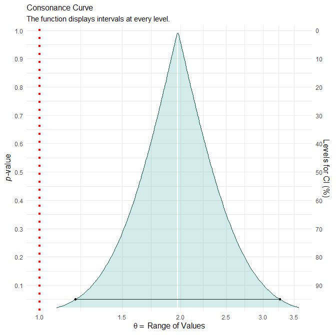
The point estimate for the odds ratio of finding the phone reminder useful is 1.97 and the associate 95% confidence interval is 1.19 to 3.26. The confidence curve is shown below.
Would an interpretation like the one below work for Example 1?
The ratio of odds of finding the phone reminder useful for females relative to males was estimated to be 1.97 (95% confidence interval: 1.19 to 3.26; p = 0.008). Since this estimated ratio and the associated P-value function both lie above 1 (which corresponds to equal odds), the study provides evidence that females have higher odds of finding the phone reminder useful compared to males. Furthermore, the 95% confidence interval indicates that the study was most compatible at the 95% confidence level with females having odds of finding the phone reminder useful that were anywhere from 19% to 226% higher than those for males.
Example 2:
This example concerns a binary logistic regression model where Y = whether or not the study subject finds a phone reminder useful and X = whether or not study subject was assessed by a physician before a threshold date. (Y is coded as before so that 1 stands for useful and 0 for not useful; X is coded as 0 if assessment date falls before the threshold date and 1 otherwise).
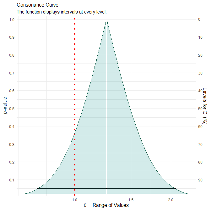
The point estimate for the odds ratio of finding the phone reminder useful is 1.26 and the associate 95% confidence interval is 0.77 to 2.06. The confidence curve is shown below.
Would an interpretation like the one below work for Example 2?
The ratio of odds of finding the phone reminder useful for those assessed by a physician after the threshold date relative to those assessed before it was estimated to be 1.26 (95% confidence interval: 0.77 to 2.06; p = 0.363). Since this estimated ratio and most of the associated P-value function lie above 1 (which corresponds to equal odds), the study provides evidence that those assessed by a physician after the threshold date have higher odds of finding the phone reminder useful compared to those assessed before that date. However, the study cannot dismiss, with a high amount of confidence, the possibility that those assessed by a physician after the threshold date have lower odds of finding the phone reminder useful. In particular, the 95% confidence interval indicates that the study was most compatible at the 95% confidence level with subjects assessed by a physician after the threshold date having odds of finding the phone reminder useful that were anywhere from 23% lower to 106% higher than those corresponding to subjects assessed before that date.
For the last statement in the above, I used that (0.77 - 1) x 100% = -23% and (2.06 - 1) x 100% = 106%.
Example 3:
This example concerns a binary logistic regression model where Y = whether or not the study subject finds a phone reminder useful and X = whether or not the study subject lives alone in their home. (Y is coded as before so that 1 stands for useful and 0 for not useful; X is coded as 0 for alone and 1 for not alone; alone is treated as the reference.)
The point estimate for the odds ratio of finding the phone reminder useful is 1.09 and the associate 95% confidence interval is 0.56 to 2.03. The confidence curve is shown below.
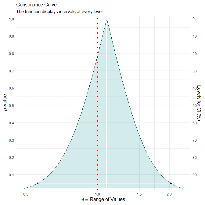
I searched the literature but couldn’t find any explicit example of interpretation of a confidence curve that covers this type of scenario, so here I am stumped as to how to report the results. (All examples I could find are along the lines captured by my Examples 1 and 2.) I would really appreciate if someone could offer a valid interpretation for this specific scenario.
Note
The above plots were created with the concurve package in R, which includes a curve_gen() function. Here is the generic R code I used to create them:
install.packages("remotes")

remotes::install_cran("pbmcapply", force = TRUE)
remotes::install_cran("concurve", force = TRUE)

library(concurve)
library(pbmcapply)

model <- glm(Y ~ X,
                  data = mydata,
                  family=binomial(link="logit"))

summary(model)

round(exp(coef(model)),2)
round(exp(confint(model)),2)

model_con <- curve_gen(model = model,
                                         var = "X",
                                        method="glm",
                                        steps = 100,
                                        table = TRUE)

 model_con

 model_consonance <- model_con[[1]]
 model_consonance$lower.limit <- exp(model_consonance$lower.limit)
 model_consonance$upper.limit <- exp(model_consonance$upper.limit)


 model_consonance_curve <-
   ggcurve(model_consonance,
                 measure = "ratio",
                 type="c",
                 nullvalue = TRUE)
When I downloaded the Github version of the concurve package, it wouldn’t show the vertical line corresponding to the null value (i.e., OR = 1), so I had to force the line to be shown using the R code below:
library(ggplot2)

model_consonance_curve +
  geom_vline(xintercept = 1, linetype=3, colour="red", size=1.5)
Also, note that I manually exponentiated the endpoints of the confidence limits produced by curve_gen() to get what I think should have been plotted in the confidence curve, rather than the default plotted by the concurve package.