How to use p-values when sample sizes are not fixed

Scenario:

  • a minimum sample size is calculated
  • a digital survey is opened, parcipants are invited to fill it in
  • procedure: “We’ll have the survey open for 30 days and stop then, unless there’s insufficient response, in which case we’ll send a reminder to potential respondents to please fill in the survey. Then we wait for another 10 days”

Let’s say you need at least 350 respondents. After 30 days you look and you are happy, because 389 people filled in the survey.

Question: can you use a normal p-value in this case? I say no. AFAIK a p-value for N=389 is calculated as follows:
- draw (hypothetically) endless samples of N=389 from a population
- calculate the relevant statistic (let’s say the t statistic) for each sample
- calculate the sampling distribution for these samples
- compare the actual sample to this sampling distribution
- conclude (e.g.) “my sample falls in the 5% most extreme values. My p-value is 0.05”

Contrast this to our scenario: Calculate the p-value for a sample of 389, where the sampling procedure is: “gather data during 30 days, unless we need 10 more days”. Here the steps are as follows:
- draw endless samples from a hypothetical population using the above procedure. The draws will have varying sizes, some will be N=389, others will be smaller, or bigger, because each time a different number of “respondents” will have “participated”
- calculate the relevant statistic (let’s say t) for each sample
- make the sampling distribution for these samples
- compare you actual sample to this sampling distribution
- conclude (e.g.) “my sample falls in the 5% most extreme values. My p-value is 0.05”

^^ in order to do this you’d have to simulate these draws. For that you need, I think, to assume two distributions:

  • the distribution of the parameter you’re intersted in (typically a normal distribution is assumed)
  • the distribution of the propensity of subjects to participate to these kind of surveys within a period of 30 + 10 days parameter (perhaps a Poisson distribution?)

Am I onto something? Or am I seeing ghosts?
Anybody knows a good paper on this problem?

Thanks!
1 Like

Get rid of significance testing and go with a hierarchical model with partial pooling. Low sample sizes will be closer to the population distribution (less certain)

You’re already thinking about simulating data, which is great. It’s an awesome way to make sure your thinking and modeling are aligned

1 Like

Frequentist operating characteristics (type I error probability and confidence interval coverage) are modified by sequential strategies. The Bayesian approach is simpler, as simulated here.

2 Likes

Hi,

I am a bit confused here.

I don’t see any indication that multiple (sequential) hypothesis tests are being performed in the scenarios described if I read correctly, only that the final sample size might change, based upon how long enrollment is permitted to proceed, conditional on the target sample size. Whatever the final sample size is at the end of the study, you perform a single test at that time.

We commonly see that scenario in clinical trials, where an a priori power/sample size calculation/simulation is performed, to yield the target sample size, based upon the presumptions around effect sizes, target alpha and power.

So, for example, let’s say that your a priori sample size is defined to be 350, to coincide with the description here.

It is common that the following will occur:

  1. You make some presumption about dropout rates, and increase the enrollment sample size accordingly, to account for the dropouts, so you still have at least your target sample size at the end of the study. That can be commonly 10% - 15%. So you adjust your target sample size to say 400 to use round numbers. Thus, your final sample size at the end of the study is likely to be above 350 and the actual final evaluable sample size will be dependent upon the actual dropout rate observed. So here, your final evaluable sample size might be anywhere from roughly 350 to 400.

  2. Enrollment for the study will take longer than projected (all the time in my experience), so the sponsor extends the enrollment accordingly. You still cutoff your enrollment when your adjusted target is hit, but the actual timeline will vary from your original estimate. Depending upon what happens, it is entirely possible that the sponsor might decide to stop enrollment at some point in time when it becomes clear that diminishing returns comes into play. That might result in something less than the target 400 being enrolled, however, ideally above the 350 original estimate.

Once you have completed the study, the a priori power/sample size estimates are largely irrelevant, with the possible exception of wanting to gain some insights into post hoc power, strictly in the event of a non-significant test at the end of the study.

If, on the other hand, sequential tests are being performed as Frank describes, then one would indeed want to consider group sequential methods/alpha spending rules in a frequentist framework, and those should be specified in the protocol a priori.

2 Likes

I already received some great insights elsewhere, that I’ll gladly share. Hope it’s useful to other readers.

I still have trouble grasping it, I admit - I feel dumb.

“So (1) fixed N design; (2) fixed time design. I recall seeing an explanation that it didn’t matter, but not sure. p seems uniform under H0 for all N”

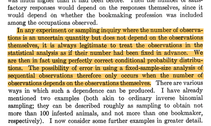
“As long as the time is independent of the ES, a conditional frequentist would just condition on N, and hence it would be the same as the fixed N approach.”

This paper takes the same stance:

Source: (scihub for the win :+1:) https://www.jstor.org.sci-hub.tw/stable/3001665

So: fixed time or fixed N, it doesn’t matter. Sounds logical, right? But then John Kruschke comes along:

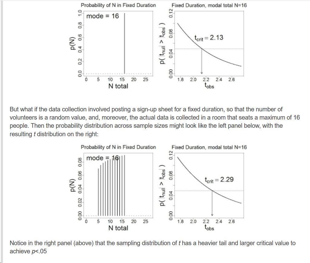
Conclusion: p-values differ depending on the sampling plan (same data, different intentions). This was also my original thought and the reason for bringing up this topic.

Response by Richard Morey:

“of course. But that doesn’t change the fact that N is ancillary.”

Sure, θ doesn’t depend on N, and neither on time: both N and time are ancillary. But my question is, can you use fixed time and fixed N interchangably? (if I am missing the point, please tell me! I feel terribly dumb but I have trouble wrapping my head around this. Enlighten me please!)

Per advice of Richard Morey I started to read these blog posts on conditioning https://normaldeviate.wordpress.com/2013/01/06/to-condition-or-not-to-condition-that-is-the-question/

And this discussion ensued on Twitter:

“Interesting thing about “paradox” Kruschke discusses, in which 2 ppl assume different sampling rules for same data, is not that one is right and one wrong. It’s that both are “right” on average (nominal alpha maintained) even though they might disagree in specific experiments (!)”

“…but: if you don’t condition you end up risking identifiable, relevant subsets where you know alpha is higher/lower than average, even though on average you know it is alpha. Many (going back to Fisher) would consider it wrong to report average alpha in those cases.”

“this is also related to paradoxes with CIs / CI fallacies …Also see the debate over the Behrens–Fisher problem.”

OK. I suppose what is meant is that CI’s have the well know pitfall that you can’t use the average coverage % to make a statement about in individual interval.

But now I still don’t understand why I can use p-values that stem from (conditioning on N) simulations in a (conditioning on time) setting. Anybody can shed some light on this? THANKS!

2 Likes