We are developing a prognostic model for cognitive development in very preterm infants using advanced MRI scans. To achieve this, we used three types of MRI information: functional connectivity (FC), structural connectivity (SC), and morphometry. Additionally, we incorporated clinical data to enrich the model. This resulted in high-dimensional data with more than 1,000 features for each subject, making model development challenging. Therefore, we needed to perform data dimension reduction.
We selected non-negative matrix factorization (NMF) for feature extraction because it facilitates the identification of statistically redundant subgraphs, allowing for overlapping and flexible co-occurrence of components. NMF’s non-negative constraints also ease the interpretability of the subgraphs as additive, positively contributing elements. We applied NMF separately to the SC and FC graph measures. Prior to modeling with NMF, the morphometry data (which included some variables with negative values) were logarithmically transformed and subsequently subjected to Min-Max scaling to meet the algorithmic assumptions of NMF.
After applying NMF to the SC, FC, and morphometry data separately, the dimensions were reduced to 31 for SC variables, 29 for FC variables, and 26 for morphometry variables. We then added 6 clinical biomarkers, 1 cMRI injury, and age at scan (a total of 94 variables).
To develop and evaluate the models, we used bootstrap optimism correction validation and kernel-based SVM. For this model, we used the ANOVA kernel. The bootstrap optimism correction evaluation involved the following steps:
- Develop the model M1 using whole data
- Evaluate the performance of M1 using whole data and ascertain the apparent performance (AppPerf).
- Generate a bootstrapped dataset with replacement
- Develop model M2 using bootstrapped dataset (applying the same modeling and predictor selection methods, as in step 1).
- Evaluate M2 using bootstrapped dataset and determine the bootstrap performance (BootPerf).
- Evaluate M2 using whole data and determine the test performance (TestPerf).
- Calculate the optimism (Op) as the difference between the bootstrap performance and test performance: ( Op=BootPerf-TestPerf) .
- Repeat Steps 3 through 7 for nboot times (n=500 ).
Average the estimates of optimism in step 8 and subtract the value from the apparent performance (step 1) to calculate the optimism-corrected performance estimate for all relevant prognostic test properties.
For recalibration this model, we did the following steps:
- Develop and evaluate the Apparent model using Whole data
- Resample the data with replacement to generate the bootstrap data
- Develop and evaluate the bootstrap model using bootstrap data
- Develop and apply the recalibration machine of outcome of bootstrap model
- Evaluate the bootstrap model using whole data to achieve the test outcome.
- Apply the recalibration machine that developed in step 4 on test outcome
- Do the steps 2 to 6 for number of bootstrapping (n=500)
To develop the recalibration machines, we used the following methos:
- Simple linear recalibration
- Piece wise linear recalibration
- Nonlinear recalibration (using Generalized additive models)
- Nonlinear recalibration (using Generalized Linear Models)
- Isotonic recalibration
- Quantile mapping
The calibration plot of this model without recalibration was as bellow:
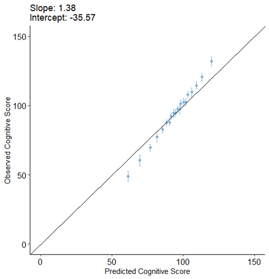
After applying the above recalibration methods, we got the following results:
Table 1. Comparing slope and intercept of test outcome after recalibration using different methods
| method |
slope |
intercept |
| Simple linear recalibration |
1.37 |
-34.43 |
| Piece wise linear recalibration |
1.27 |
-24.76 |
| Nonlinear recalibration (using Generalized additive models) |
1.29 |
-27.11 |
| Nonlinear recalibration (using Generalized Linear Models) |
1.30 |
-27.91 |
| Isotonic recalibration |
1.38 |
-35.29 |
| Quantile mapping |
1.29 |
-26.66 |
I wondered if there is a method to improve this recalibration and make the model closer to ideal model (intercept=0 and slope=1)?
I may have missed it but I didn’t see the number of observations or the distribution of Y. Those are all-important. If the effective sample size is not at least around 2000, the amount of overfitting expected may easily make the bootstrap underestimate overfitting. 100 repeats of 10-fold CV may be called for.
You are right to use data reduction; I’m not familiar with the matrix factorization approach. But it does strike me that the chances of all this being meaningful are low without injection of biological knowledge into the data reduction process.
Dear Dr. Harrell,
Thank you for your response. I was wondering if you could kindly share a reference that provides a mathematical proof showing that a small sample size causes the bootstrap optimism correction to underestimate overfitting?
It’s not the small sample size on its own. It’s when N << p. Sorry I don’t have a reference handy but there is a good one showing that intensive cross-validation is still unbiased in that case.
Dear Prof. Harrell,
I am relatively new to calibration methods applied in survival analysis. I believe I understand your approach to calibration and have successfully implemented it using simulations.
Although this thread is not specifically about survival analysis, it is relevant to my broader question. Why, unlike the evaluation of calibration methods in Machine Learning—where the focus is on how well-calibrated models can predict new (test) data—do your analyses focus on how well a model is calibrated? Furthermore, to address this question, a calibration model (e.g., hazard regression) is often used, but its validity is not always established.
For example, an excellent paper by Austin, Harrell, et al., Graphical calibration curves and the integrated calibration index (ICI) for survival models (2020), recommends ICI for comparing competing survival models but does not discuss the goodness of calibration fit
Isn’t it equally important to evaluate how well a calibrated model predicts new observations? Thank you for your attention
There are a few issues here. One is that I don’t use calibration to check for goodness of fit, but rather use directed assessments related to linearity and additivity. Second, I do emphasize calibration assessment consistent with accurate predictions of new observations, by emphasizing overfitting-corrected calibration curves.
Dear Prof. Harrell, Thank you very much for your quick reply and for clarifying that you rely on direct assessments of model structure (e.g., linearity, additivity) rather than calibration curves for overall goodness of fit, and that you use overfitting-corrected calibration curves primarily to ensure accurate prediction for new observations.
I’d like to revisit the calibration step specifically. In some applications, especially high-dimensional random-forest–based survival models, one my add a Cox-spline calibration layer (e.g., rcs(forest.time1, 3)) to refine the raw forest predictions. My question focuses on how to assess that calibration model’s goodness of fit—in other words, how well the combined “random forest + calibration layer” approach performs, beyond simply comparing calibrated vs. raw predictions.
In the “Graphical calibration curves and the integrated calibration index (ICI) for survival models” paper, the ICI is a useful measure of alignment between predicted and observed outcomes, but it does not always confirm that the calibration model is valid if it merely shows how far calibrated predictions have moved from the raw ones. So for an external dataset (with known outcomes), how best should one formally verify that this two-step approach (forest + calibration) is delivering genuinely improved calibration? Is it simply a matter of plotting overfitting-corrected calibration curves on the external data, or do you recommend additional methods (e.g., plotting partial residuals, recalculating an ICI with respect to observed outcomes, etc.)? " Thank you very much!
1 Like
Good questions. When a black box prediction tool is used, sometimes we must rely on overall accuracy measures such as 0…9 quantile of calibration error, Brier score, root mean squared prediction error, etc. For these you can correct them for overfitting using repeated cross-validation or the bootstrap. I suppose for RF you can check calibration in specific subsets of observations to check fit in more detail. But usuall the overall calibration in RF is such a disaster that you don’t spend time carrying it any further.
Thank you once again for your answers and your service to the community. I spent some time learning your RMS calibrate procedure and also implemented Austin & Harrell’s code for the comparison of 3 models, RSF, Generalized RF, and CoxPH. I am not concerned with overfitting since I have 3 datasets for training, calibration, and testing, respectively, each with 2000 observations and from 6 to 24 variables. The calibration error (ICI) and its 90% are relatively small. In fact, they might be so small that the errors after calibration (using the phare prediction model) are not getting smaller and, in some cases, are even higher. I am taking it as evidence that I should not be worried about the calibration of any of the three models.
1 Like
That sounds good. I just suggest supplementing what you’ve done with 0.95 confidence bands (compatibility intervals) for the calibration curves.