Interpreting and visualizing a Cox model for prognostic factors

I’m analyzing TCGA survival data to understand the prognostic importance of biomarkers from genes G1 and G2. Two different markers are measured for each gene: copy number (cnv) and expression (rna). I’ve fitted a pre-specified model which includes the genetic markers and other prognostic factors available from the data:

test.model <-  fit.mult.impute(Surv(OS.time, OS) ~ rcs(age, 3) + gender + tobacco_smoking_history +
                                radiation_therapy + G1.cnv + G2.cnv + rcs(G2.rna, 3) * rcs(G1.rna, 3), 
                              cph, imp, data = patients)

Checking the ANOVA for the model yields:

               Wald Statistics          Response: Surv(OS.time, OS) 

 Factor                                         Chi-Square d.f. P     
 age                                             2.89       2   0.2359
  Nonlinear                                      2.71       1   0.0999
 gender                                          3.73       1   0.0533
 tobacco_smoking_history                         2.38       4   0.6670
 radiation_therapy                               1.42       1   0.2330
 G1.cnv                                          0.70       4   0.9519
 G2.cnv                                          0.54       4   0.9700
 G2.rna  (Factor+Higher Order Factors)          14.06       6   0.0290
  All Interactions                              13.89       4   0.0077
  Nonlinear (Factor+Higher Order Factors)        6.42       3   0.0930
 G1.rna  (Factor+Higher Order Factors)          14.36       6   0.0259
  All Interactions                              13.89       4   0.0077
  Nonlinear (Factor+Higher Order Factors)        2.34       3   0.5040
 G2.rna * G1.rna  (Factor+Higher Order Factors) 13.89       4   0.0077
  Nonlinear                                      6.91       3   0.0749
  Nonlinear Interaction : f(A,B) vs. AB          6.91       3   0.0749
  f(A,B) vs. Af(B) + Bg(A)                       0.03       1   0.8723
  Nonlinear Interaction in G2.rna vs. Af(B)      5.80       2   0.0550
  Nonlinear Interaction in G1.rna vs. Bg(A)      0.85       2   0.6534
 TOTAL NONLINEAR                                 9.65       6   0.1402
 TOTAL NONLINEAR + INTERACTION                  15.57       7   0.0294
 TOTAL                                          27.56      24   0.2792

The small p-values for G1.rna, G2.rna, and the interaction(0.0259, 0.0290, 0.0077 respectively) suggest to me that the expression markers for each gene may have prognostic value, but I’m concerned that the model’s overall p-value is rather large (0.2792).

I’ve further assessed the importance of G1 and G2 expression with the likelihood ratio test and
the adequacy index:

subset.model <- fit.mult.impute(Surv(OS.time, OS) ~ rcs(G2.rna, 3) * rcs(G1.rna, 3),
                                                  cph, imp, data = patients)
lrtest(subset.model, full.model)
A <- 1 - subset.model$stats['Model L.R.'] / full.model$stats['Model L.R.']

lrtest p-value = .1 and A = .42, providing some (although weaker) evidence that G1 and G2 expression may be prognostic.

How should I interpret these contrary results? Is it possible to reconcile the overall model’s large p-value with the individual variables smaller p-values, or must I conclude more data is needed to make any conclusions? In general, if the overall model’s p-value is large, should any individual p-values be ignored?

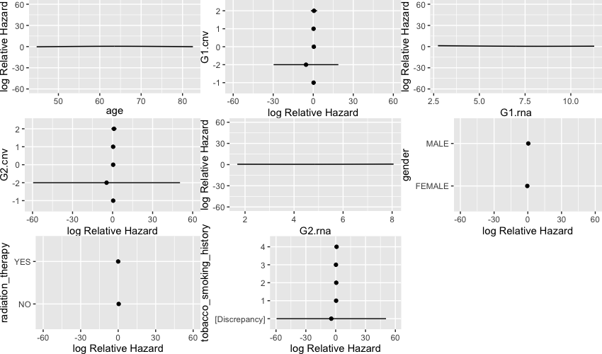
Additionally, I’m trying to visualize the relationship between G1.rna and G2.rna. When I visualize all the predictors the plots seem rather flat:

ggplot(Predict(test.model))

Visualizing only G1.rna with certain values of G2.rna is much less flat:

ggplot(Predict(test.model, G1.rna, G2.rna = c(0, 3, 6, 9)))

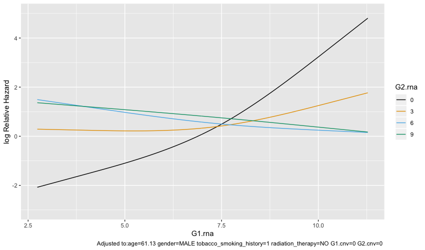
I see that the the second plot says adjusted to several factors while the first plot doesn’t. Are the curves from ggplot(Predict(test.model)) averaged across all conditions while ggplot(Predict(test.model, G1.rna, G2.rna = c(0, 3, 6, 9))) shows the curve only for specific condition? If so, which plot should I be showing?

2 Likes

i wouldn’t look at the overall model p-value. Regarding the change in p-value for g1 and g2, is it due to type I v type II sums of squares? I’m not familiar with the software you’re using (i guess it’s R). Something is certainly wrong with the plot. I would calculate it by hand if you don’t know what R is doing

edit: I just saw the final plot, looks better!

1 Like

Tomas you’re looking at this is an excellent way. A complication is that not all the statistics coming from cph are worked out for multiple imputation. The LR test and measures of predictive discrimination come only from the last imputation unfortunately. It’s best to stick with anova Wald tests which use all the imputations. You might do a chunk test for combined effects of both rna factors, e.g. anova(test.model, G1.rna, G2.rna) and also do an anova combining these with cnv variables to get an overall multiplicity-adjusted test of all G variables.

How many events are in the dataset?

In terms of large overall P-value this is a bit of concern but needs to be more directly addressed by computing some measures of total model predictive discrimination. You might compute the variance of X\hat{\beta} for each imputation and average all those variances, and do likewise for c-indexes using rcorr.cens or the faster function for this in the survival function.

1 Like

I wasn’t aware of those cph limitations, thanks for the heads up. I’m working with a very small dataset of 185 patients and 77 events. I realize with so few events the large p-values are to be expected unless the effect size is huge.

Both chunk tests offer some evidence for G1 and G2 rna expression as useful predictive markers

anova(test.model, G2.rna, G1.rna)
              Wald Statistics          Response: Surv(OS.time, OS) 

 Factor                                   Chi-Square d.f. P     
 G2.rna  (Factor+Higher Order Factors)    13.74      6    0.0327
  All Interactions                        13.40      4    0.0095
  Nonlinear (Factor+Higher Order Factors)  6.24      3    0.1003
 G1.rna  (Factor+Higher Order Factors)    13.69      6    0.0333
  All Interactions                        13.40      4    0.0095
  Nonlinear (Factor+Higher Order Factors)  1.93      3    0.5874
 TOTAL NONLINEAR                           6.92      5    0.2263
 TOTAL                                    13.99      8    0.0820
anova(test.model, G1.rna, G2.rna, G1.cnv, G2.cnv, G2.rna * G1.rna)
     Wald Statistics          Response: Surv(OS.time, OS) 

 Factor                                         Chi-Square d.f. P     
 G1.rna  (Factor+Higher Order Factors)          13.69       6   0.0333
  All Interactions                              13.40       4   0.0095
  Nonlinear (Factor+Higher Order Factors)        1.93       3   0.5874
 G2.rna  (Factor+Higher Order Factors)          13.74       6   0.0327
  All Interactions                              13.40       4   0.0095
  Nonlinear (Factor+Higher Order Factors)        6.24       3   0.1003
 G1.cnv                                          0.73       4   0.9475
 G2.cnv                                          0.53       4   0.9705
 G2.rna * G1.rna  (Factor+Higher Order Factors) 13.40       4   0.0095
  Nonlinear                                      6.24       3   0.1006
  Nonlinear Interaction : f(A,B) vs. AB          6.24       3   0.1006
  f(A,B) vs. Af(B) + Bg(A)                       0.00       1   0.9774
  Nonlinear Interaction in G2.rna vs. Af(B)      5.22       2   0.0734
  Nonlinear Interaction in G1.rna vs. Bg(A)      0.82       2   0.6650
 TOTAL NONLINEAR                                 6.92       5   0.2263
 TOTAL NONLINEAR + INTERACTION                  13.93       6   0.0305
 TOTAL                                          17.79      16   0.3366

I’ve managed to use survConcordance to compute the c-index for the full and subset model:

concordance(Surv(OS.time, OS) ~test.model$linear.predictors)
n= 185 
Concordance= 0.3497 se= 0.03639
concordant discordant     tied.x     tied.y    tied.xy 
      2672       4968          0          2          0 
concordance(surv.obj ~ subset.model$linear.predictors)
n= 185 
Concordance= 0.3573 se= 0.03735
concordant discordant     tied.x     tied.y    tied.xy 
      2730       4910          0          2          0 

I would assume that subset.model's slightly better c-index is due to the c-index not being sensitive enough to compare performance between models. Neither c-index from survConcordance seems to match the D_{xy} from the model output

full.model
                      Model Tests       Discrimination    
                                           Indexes        
 Obs        185    LR chi2     31.80    R2       0.162    
 Events      77    d.f.           24    Dxy      0.294    
 Center 11.0456    Pr(> chi2) 0.1336    g        1.028    
                   Score chi2  31.21    gr       2.797    
                   Pr(> chi2) 0.1490                      

Using D_{xy} = 2 (c - \frac{1}{2}), I would get a D_{xy}= 2(.3497-.5) = -3.006, not 0.294.

subset.model
                   Model Tests       Discrimination    
                                        Indexes        
 Obs     185    LR chi2     18.35    R2       0.097    
 Events   77    d.f.           16    Dxy      0.270    
 Center 6.58    Pr(> chi2) 0.3099    g        0.798    
                Score chi2  17.44    gr       2.229    
                Pr(> chi2) 0.3634                      

Similarly, D_{xy} = 2(0.3573 - .5) = -.2854, not 0.270. Is there a reason these numbers don’t match?

After doing some reading on Type I vs Type II sums of squares, I’m assuming anova in rms uses Type II although I couldn’t find any information about this in the documentation. What’s your intuition for not looking at the overall model?

Note I used concordance instead of survConcordance because there was a warning that survConcordance has been deprecated and suggested using concordance instead. Interestingly they yield different c-indexes:

survConcordance(surv.obj ~ test.model$linear.predictors)
Call:
survConcordance(formula = surv.obj ~ full.model$linear.predictors)

  n= 185 
Concordance= 0.6502618 se= 0.03804693
concordant discordant  tied.risk  tied.time   std(c-d) 
  4968.000   2672.000      0.000      2.000    581.357 
concordance(surv.obj ~ test.model$linear.predictors)
Call:
concordance.formula(object = surv.obj ~ full.model$linear.predictors)

n= 185 
Concordance= 0.3497 se= 0.03639
concordant discordant     tied.x     tied.y    tied.xy 
      2672       4968          0          2          0 

Looks like concordance = 1- survConcordance

1 Like

i have never looked at the p-value for a full model, but my background is mostly RCTs. i suspect you want something else ie ‘predictive discrimination’ mentioned by @f2harrell Although i’m not sure you’re building a model for prediction, you just want to evaluate the predictive ability of the two markers(?)

1 Like

Ah yes, I missed that. It turns out my concordance call was incorrectly formatted. The way I call concordance(surv.obj ~ test.model$linear.predictors) must flip the interpretation because concordance(test.model) gives the same c-index as survConcordance. This only works with non-imputed models though - concordance doesn’t seem to know how to handle an imputed model.

Yes, I’m not interested in building a prediction model per se - there isn’t enough data/covariates to build a model that will externally validate and be useful in clinic. Due to the limiting circumstances, I’m more interested to know if there is any evidence to suggest these genes be further studied as potential prognostic factors that can be included in future models.

In that regards, I’m interested in showing that these genes do improve predictive discrimination, but I’ve read that measures like the c-index aren’t sensitive enough and it’s better to use likelihood ratio p-values and adequacy indexes. I’m open to other suggestions though if you think there are better ways to evaluate predictive ability.

You can’t use an interaction term in anova( ) with asterisk. anova automatically pools all the needed terms, i.e., if you say anova(a,b) you’ll get any interactions involving either a or b.

Your pooled test with 8 d.f. for G*.rna has P=0.08. This is a perfect multiplicity adjustment. So your model is not ready for prime time. You might even argue that you should pool the cnv variables with this chunk test.

1 Like

That makes sense, thank you everyone for all the help!