Is it valid to use "withdrew from study" in a mixed model to help with dropout bias in longitudinal data?

[Evan]

Consider the hypothetical dataset where a number of study participants have no change over time in a particular outcome, but their probability to drop out of the study is related to the baseline value of the outcome. How can I make sure that this dropout doesn’t bias my mixed model to incorrectly fit an effect of time? Can I include an indicator for whether a subject dropped out as a covariate? Or is that problematic in a way I’m not realizing?

I’m open to more general solutions, in addition to getting an answer to the main question. I have already done some reading to figure this out, and found some possible leads such as inverse probability weighting and doubly robust generalized estimating equations. However, I tried one R package for the latter (wgeesel), and it doesn’t seem to be doing what I expected. It’s also a completely new framework for me - I would prefer to stick with mixed models if possible.

Here is some code & plots that illustrates the issue (omitting model summaries):

library(nlme)
library(tidyverse)

n.participants = 1000
max.fu = 4

set.seed(42)

df = tidyr::crossing(
  subjid = 1:n.participants,
  elapsed = 0:max.fu
) %>%
  dplyr::mutate(
    hidden = dplyr::case_when(
      subjid < n.participants/2 ~ 1,
      subjid >= n.participants/2 ~ 2
    ),
    outcome = hidden + rnorm(n.participants)
  ) %>%
  dplyr::filter(
    elapsed <= max.fu*hidden/2
  )

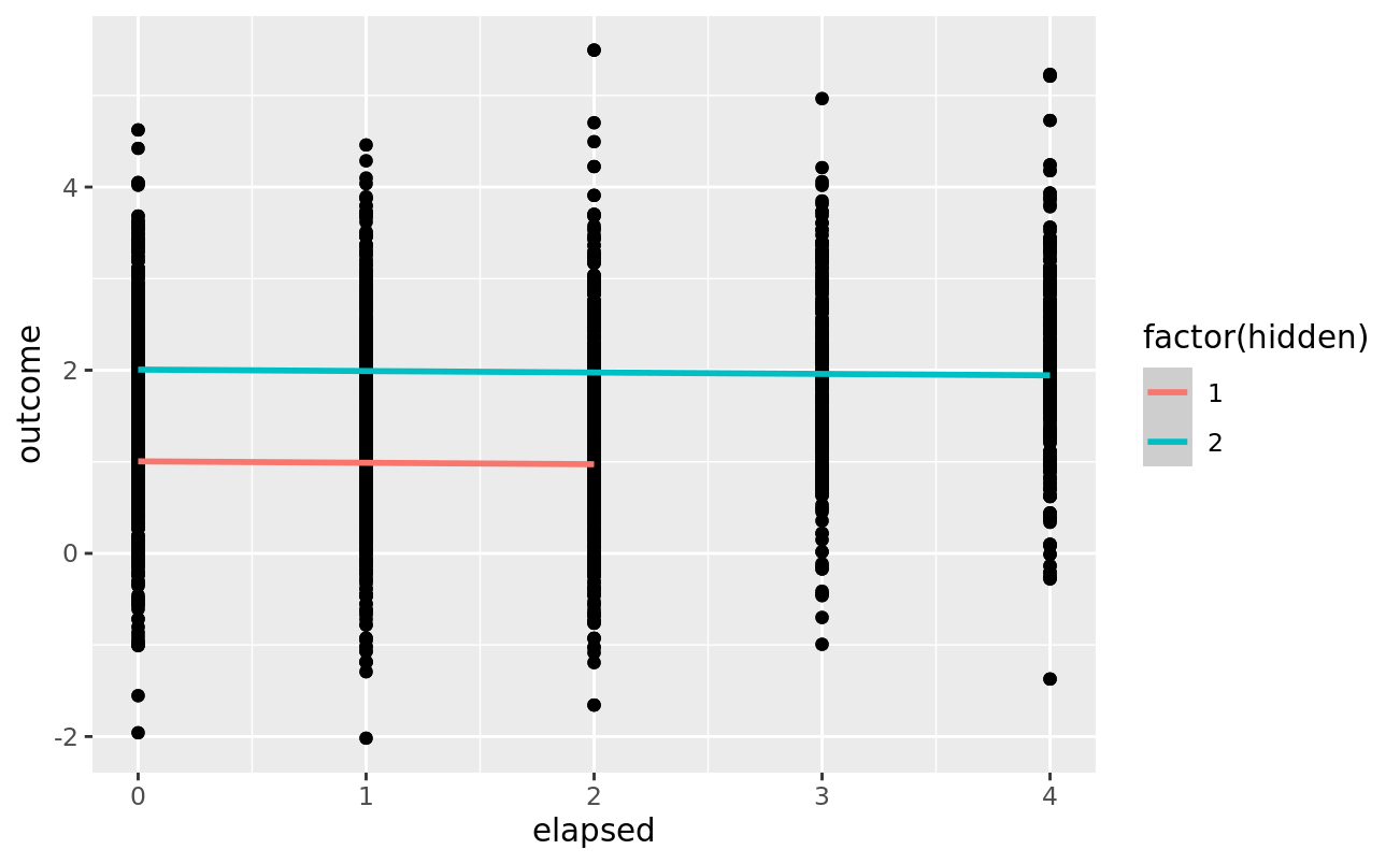
df %>%
  ggplot(aes(x = elapsed, y = outcome, color = factor(hidden))) +
  geom_point() +
  geom_smooth(method = "lm", formula = "y ~ x")

When this is fit without the “hidden” variable which dictates baseline & dropout, I get an effect of time:

model1 = df %>%
  nlme::lme(
    outcome ~ elapsed,
    random = ~1 | subjid,
    data = .
  )

df$fit1 = predict(model1)

df %>%
  ggplot(aes(x = elapsed, y = outcome)) +
  geom_point() +
  geom_smooth(
    aes(y=fit1, color = hidden),
    method = "lm", formula = "y ~ x"
  )

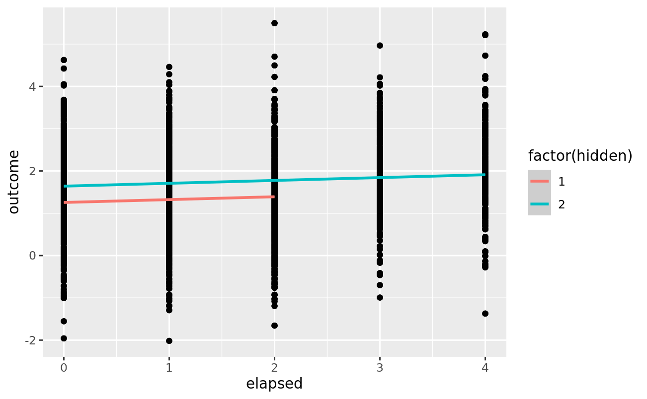
Including the “hidden” covariate, the effect goes away:

model2 = df %>%
  nlme::lme(
    outcome ~ elapsed + hidden,
    random = ~1 | subjid,
    data = .
  )

df$fit2 = predict(model2)

df %>%
  ggplot(aes(x = elapsed, y = outcome)) +
  geom_point() +
  geom_smooth(
    aes(y=fit2, color = factor(hidden)),
    method = "lm", formula = "y ~ x"
  )

[js592]

You might have better luck treating it as an absorbing state in a Markov type model

[sscogges]

Are you concerned about the situation where the baseline value of the outcome influences drop-out, or where you have a (potentially unmeasured) covariate that influences both the outcomes and drop-out? What you’ve simulated here corresponds to the latter, not the former. In your simulations, the probability of dropping out is determined completely by the hidden variable. Thus, baseline value of the outcome is not really a cause of missingness.

More technically, in your simulations your data are Missing at Random (MAR) conditional on hidden, but not the baseline value of the outcome. Your simulations correctly show that, to avoid bias from missing data, you have to account for hidden in your analysis in order to meet the MAR assumption. This will be the case regardless of whether you use mixed models, propensity score weighting, etc. E.g. a propensity score weighting approach would have to include hidden in the estimation of the propensity score.

Mixed models do, under certain conditions, account for missing outcomes/drop-out that is dependent on previously observed values of the outcome. But that is different from what you’ve simulated here.

[Evan]

@sscogges I didn’t suppose that the causality of the dropout was too important, in the context of the question, which is whether I can use the dropout itself as a covariate. How would the cause of the dropout (the outcome itself vs. some observed or unobserved covariate) affect the validity of my proposed strategy?

[f2harrell]

If dropout tendency is a combination of being completely random and a function of known measurements (baseline or Y from previous times) then you have missing at random and just need to analyze all available data using standard likelihood (not GEE) approaches.

[Evan]

Thanks @f2harrell - are you able to comment specifically on the strategy of using the “withdrew” indicator as a covariate? In my toy example, adding baseline as a covariate doesn’t do much to remove the bias, whereas the “withdrew” indicator appears to remove it completely. In case it matters, I will not be inferring dropout from the outcome data in my actual analysis - there is an independent variable for this at the participant level.

Naive model, beta_elapsed = 0.067 +/- 0.012:

model.naive = df %>%
  nlme::lme(
    outcome ~ elapsed,
    random = ~1 | subjid,
    data = .
  )

model.naive %>% summary() %>% print()

Model with baseline, beta_elapsed = 0.064 +/- 0.012:

model.baseline = df %>%
  dplyr::group_by(subjid) %>%
  dplyr::mutate(baseline = outcome[elapsed == 0]) %>%
  dplyr::ungroup() %>%
  nlme::lme(
    outcome ~ elapsed + baseline,
    random = ~1|subjid,
    data = .
  )

model.baseline %>% summary() %>% print()

Model with withdrawal indicator, beta_elapsed = -0.016 +/- 0.013 (equivalent to model 2 above, but refactoring not to use hidden, in case that is confusing):

model.dropout = df %>%
  dplyr::group_by(subjid) %>%
  dplyr::mutate(withdrew = any(elapsed == max.fu)) %>%
  dplyr::ungroup() %>%
  nlme::lme(
    outcome ~ elapsed + withdrew,
    random = ~1|subjid,
    data = .
  )

model.dropout %>% summary() %>% print()

[f2harrell]

Putting a post-time-zero variable into the baseline model creates an uninterpretable result

[Evan]

@f2harrell do you mean the coefficient for “withdrew” is uninterpretable, or rather does inclusion of the “withdrew” term render the entire model (and critically, the effect of “elapsed”) uninterpretable?

I see how the former could be true - it would be absurd to say “there is an effect of withdrawal on outcome”, given that by definition, the withdrawal is observed after the available outcome observations have been made. However, I think it would be reasonable to say “there is an association between withdrawal and outcome”, i.e., there are some unobserved factors influencing both outcome and withdrawal, and we can use withdrawal itself as a nuisance variable serving as proxy.

If you mean the latter (the whole model is uninterpretable), what would be the proper way to model this toy example (i.e., avoid the upwards bias), assuming we don’t have access to the true causal variable “hidden”?

I’d love to learn more about this concept in general, if you have links or references to textbook chapters, blog posts, and/or forum discussions. Thanks for your time!