Logistic Model Shap Analysis

Hello there,

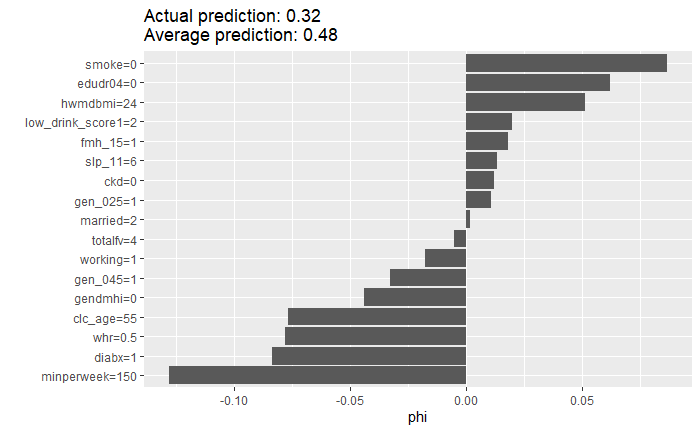
Hope everyone is doing well. I have developed and validated a logistic regression model predicting hypertension for my thesis. For a given observation, I now want to visualize the contribution of predictors with Shapley additive explanation (Shap) plots using the iml R package. I try to run the following code, but run into the error in the photo at the bottom. I believe the error has something to do with using rcs but I still want to use my model with splines, interactions, replicate weights. There’s no missing data by the way.

Would appreciate any feedback!

Thanks,
Raf

# Set final models
male_final_model <- survey::svyglm(highbp14090_adj ~ rcs(clc_age, 4) + married + edudr04 + working + gendmhi + gen_025 + gen_045 + fmh_15 + rcs(hwmdbmi, 3) + rcs(whr, 3) + low_drink_score1 + rcs(minperweek, 3) + smoke + slp_11 + totalfv + diabx + ckd + rcs(clc_age, 4)*gen_045 + rcs(clc_age, 4)*rcs(hwmdbmi, 3) + rcs(clc_age, 4)*rcs(whr, 3) + rcs(clc_age, 4)*rcs(minperweek, 3) + rcs(clc_age, 4)*smoke + rcs(clc_age, 4)*slp_11 + rcs(clc_age, 4)*diabx + rcs(clc_age, 4)*ckd + rcs(hwmdbmi, 3)*rcs(whr, 3), design = weighted_male, family = quasibinomial())

# Create the Predictor object with 'response' to get probabilities
male_explainer <- iml::Predictor$new(
  model = male_final_model,                                       # Pass the model
  data = male_data,                                               # Pass the data
  y = male_data[["highbp14090_adj"]],                             # Indicate outcome
  type = "response"                                               # Return predicted probabilities
)

# Create observation as a data frame
observation <- data.frame(
  clc_age = 62,
  married = 1,
  edudr04 = 1,
  working = 1,
  gendmhi = 1,
  gen_025 = 1,
  gen_045 = 1,
  fmh_15 = 1,
  hwmdbmi = 20,
  whr = 0.7,
  low_drink_score1 = 2,
  minperweek = 100,
  smoke = 1,
  slp_11 = 8,
  totalfv = 5,
  diabx = 1,
  ckd = 0
)

# Compute SHAP values for observation
shap_values <- iml::Shapley$new(male_explainer, x.interest = observation)

# Visualize SHAP values for observation
shap_values$plot()

image

Shap is probably not a valid method as it gives the wrong answer when predictors are correlated with each other. And whatever you do you must include a confidence interval to show how nearly impossible this task is. Consider using measures of relative explained variation I discuss in RMS chapters 4, 5, 9.

2 Likes

Hello Dr. Harrell,

Thanks for the response! Very much appreciated! I understand your view on Shap, but I should have specified earlier that I want to specifically use Shap to explain the contribution of each unique predictor to the predicted outcome, while accounting for both nonlinearity and interactions. I want to explain this contribution per unique predictor visually for a given observation (synthetic example below) and eventually for future users of my model. I also want to compute single Shap-adjusted ORs and CIs for each continuous predictor and each categorical predictor non-reference level.

image

However, as seen in my first message, iml throws an error for svyglm or lrm models. When I fit a weighted glm model with my real data, the code works but the predicted probabilities all become 0 or 1 for some reason.

I did look at partial R2s in RMS Ch 9, but would they be the optimal measure of predictor contributions for my binomial logistic model?

Would appreciate any feedback as always!

Thanks,
Rafidul

Also, it seems like the same error occurs when I try to predict the outcome on any new data. Anyone know why that could be?

> # Set final models
> male_final_model <- survey::svyglm(highbp14090_adj ~ rcs(clc_age, 4) + married + edudr04 + working + gendmhi + gen_025 + gen_045 + fmh_15 + rcs(hwmdbmi, 3) + rcs(whr, 3) + low_drink_score1 + rcs(minperweek, 3) + smoke + slp_11 + totalfv + diabx + ckd + rcs(clc_age, 4)*gen_045 + rcs(clc_age, 4)*rcs(hwmdbmi, 3) + rcs(clc_age, 4)*rcs(whr, 3) + rcs(clc_age, 4)*rcs(minperweek, 3) + rcs(clc_age, 4)*smoke + rcs(clc_age, 4)*slp_11 + rcs(clc_age, 4)*diabx + rcs(clc_age, 4)*ckd + rcs(hwmdbmi, 3)*rcs(whr, 3), design = weighted_male, family = quasibinomial())

> # Create observation as a data frame
> observation <- data.frame(
+     clc_age = 62,
+     married = 1,
+     edudr04 = 1,
+     working = 1,
+     gendmhi = 1,
+     gen_025 = 1,
+     gen_045 = 1,
+     fmh_15 = 1,
+     hwmdbmi = 20,
+     whr = 0.7,
+     low_drink_score1 = 2,
+     minperweek = 100,
+     smoke = 1,
+     slp_11 = 8,
+     totalfv = 5,
+     diabx = 1,
+     ckd = 0
+ )
> 
> predict(male_model, observation, type = "response")
Error in rcspline.eval(x, nk = nknots, inclx = TRUE, pc = pc, fractied = fractied) : 
  knots not specified, and < 6 non-missing observations

Would appreciate any feedback on any of my two coding issues!

Sincerely,
Rafidul

Optimal measures are likelihood ratio \chi^2, pseudo adjusted R^2, and the measures here. And look hard at relative explained variation and its confidence intervals described in a few places in RMS.