Reviewer comments, and a related article by Gelman and Park (http://www.stat.columbia.edu/~gelman/research/published/thirds5.pdf), got me thinking about this.
Preserving the continuous nature of a variable in data analysis is generally superior to the use of an arbitrarily discretized version thereof for 2 broad categories of reasons:
- From an analytic perspective, it maximizes statistical precision, minimizes residual confounding/bias, and respects the underlying physiology.
- For graphical purposes, It allows higher-resolution graphical displays of the effects of a variable (or interactions between them) across their full spectrum.
However, most lay audiences (including most physicians) are, for better or worse, mentally primed to interpret more familiar portrayals displaying (for example) the probability of an event across discrete bins (e.g., tertiles). I am completely aware this is a coarsened low-resolution display, particularly if there’s a lot of heterogeneity within each bin. A simple smooth line (if displaying probability across the continuum of 1 variable) or a heatmap (if across the continuum of 2 variables) would provide a more faithful depiction. That said, because of sheer unfamiliarity, you’d probably have to pause and explain these more granular resolutions to lay audiences who’re not used to seeing data depicted this way. In other words, there is a bit of a cognitive/time pricetag on the use of somewhat unfamiliar graphical displays. Some are not willing to pay said pricetags and simply want the familiar bar graphs they’re used to.
On that premise, what we’d want is a compromise that accedes to the demands of simplification (thereby sacrificing the 2nd set of advantages) but does not forsake (all of) the analytic advantages.
So I was thinking of something along these lines:
1. Build your model while preserving the continuous nature of the variables and base all of your inferential claims (e.g., added values of a given predictor or statistical interaction) on this model.
2. Provide high-resolution continuous displays for audiences who have the prerequisite ability to interpret them (or are willing to spend time/effort to learn how).
3. When discretized displays are desired by reviewers or for lay audience presentations, marginalize the predictions of your continuous model over the empirical distribution of the continuous variable within the desired discrete bins. The same approach can be applied for discretized interactions between variables
Below is an example of a logistic model with an interaction between LVEF category (usually categorized into 3 bins) and HR for predicting some binary outcome:
library(data.table)
#Sample size
n <- 2500

#Generate predictors
sex <- rbinom(n, 1, 0.5)
age <- runif(n, 40, 85)
lvef <- 100*rbeta(n, shape1 = 5, shape2 = 5) #Beta distribution with mean of 0.5 (50%)
lvef_cat <- fcase(lvef <= 40, "Low", lvef > 40 & lvef < 50, "Mid", lvef >= 50, "High")
hr <- rgamma(n, shape = 50, rate = 0.5) #Gamma distribution with a mean of 100
hr_cat <- fcase(hr < 100, "Low", hr >= 100, "High")

#Generate outcome
z <- -12 + 0.1*sex + 0.1*age + 0.01*hr + 0.01*lvef + 0.001*hr*lvef
prob <- plogis(z)
y <- rbinom(n, 1, prob)

library(rms)
#We don't know linearity apriori, so we use restricted cubic splines for the continuous model (plus a linear interaction)
glm(family = binomial, y ~ sex + rcs(age) + rcs(lvef, 4) + rcs(hr, 4) + lvef:hr) -> mcont
#And now we run the model treating LVEF as a categorical variable
glm(family = binomial, y ~ sex + rcs(age) + lvef_cat*hr_cat) -> mcat

#Summary statistics/tests
summary(mcont)
summary(mcat)
anova(mcont)
anova(mcat)


library(marginaleffects)
##Much of what follows could be simplified with lapply, but is kept expanded for clarity's sake

#Create data.frames for m1 predictions

#Comprising the low LVEF group
#With a low HR
data.frame(sex = median(sex),
           age = median(age),
           lvef = lvef[hr_cat == "Low" & lvef_cat == "Low"],
           hr = hr[hr_cat == "Low" & lvef_cat == "Low"],
           lvef_cat = "Low",
           hr_cat = "Low") -> lowef_lowhr_df

#Comprising the mid-range LVEF group
data.frame(sex = median(sex),
           age = median(age),
           lvef = lvef[lvef_cat == "Mid" & hr_cat == "Low"],
           hr = hr[lvef_cat == "Mid" & hr_cat == "Low"],
           lvef_cat = "Mid",
           hr_cat = "Low") -> midef_lowhr_df

#Comprising the high LVEF group
data.frame(sex = median(sex),
           age = median(age),
           lvef = lvef[lvef_cat == "High" & hr_cat == "Low"],
           hr = hr[lvef_cat == "High" & hr_cat == "Low"],
           lvef_cat = "High",
           hr_cat = "Low") -> highef_lowhr_df


#With a high HR
data.frame(sex = median(sex),
           age = median(age),
           lvef = lvef[lvef_cat == "Low" & hr_cat == "High"],
           hr = hr[lvef_cat == "Low" & hr_cat == "High"],
           lvef_cat = "Low",
           hr_cat = "High") -> lowef_highhr_df

#Comprising the mid-range LVEF group
data.frame(sex = median(sex),
           age = median(age),
           lvef = lvef[lvef_cat == "Mid" & hr_cat == "High"],
           hr = hr[lvef_cat == "Mid" & hr_cat == "High"],
           lvef_cat = "Mid",
           hr_cat = "High") -> midef_highhr_df

#Comprising the high LVEF group
data.frame(sex = median(sex),
           age = median(age),
           lvef = lvef[lvef_cat == "High" & hr_cat == "High"],
           hr = hr[lvef_cat == "High" & hr_cat == "High"],
           lvef_cat = "High",
           hr_cat = "High") -> highef_highhr_df

#m1 predictions, marginalizing over the distribution of LVEF within each bucket
#For a low HR
avg_predictions(mcont,
                newdata = lowef_lowhr_df) -> lowef_lowhr_pred_mcont
avg_predictions(mcont,
                newdata = midef_lowhr_df) -> midef_lowhr_pred_mcont
avg_predictions(mcont,
                newdata = highef_lowhr_df) -> highef_lowhr_pred_mcont
#For a high HR
avg_predictions(mcont,
                newdata = lowef_highhr_df) -> lowef_highhr_pred_mcont
avg_predictions(mcont,
                newdata = midef_highhr_df) -> midef_highhr_pred_mcont
avg_predictions(mcont,
                newdata = highef_highhr_df) -> highef_highhr_pred_mcont

#m2 predictions, treating each bucket as a completely separate category
#For a low HR
avg_predictions(mcat,
                newdata = lowef_lowhr_df) -> lowef_lowhr_pred_mcat
avg_predictions(mcat,
                newdata = midef_lowhr_df) -> midef_lowhr_pred_mcat
avg_predictions(mcat,
                newdata = highef_lowhr_df) -> highef_lowhr_pred_mcat
#For a high HR
avg_predictions(mcat,
                newdata = lowef_highhr_df) -> lowef_highhr_pred_mcat
avg_predictions(mcat,
                newdata = midef_highhr_df) -> midef_highhr_pred_mcat
avg_predictions(mcat,
                newdata = highef_highhr_df) -> highef_highhr_pred_mcat

#Bind their predictions together in a single data.frame to facilitate plotting
rbind(lowef_lowhr_pred_mcont,
      midef_lowhr_pred_mcont,
      highef_lowhr_pred_mcont,
      lowef_highhr_pred_mcont,
      midef_highhr_pred_mcont,
      highef_highhr_pred_mcont,
      lowef_lowhr_pred_mcat,
      midef_lowhr_pred_mcat,
      highef_lowhr_pred_mcat,
      lowef_highhr_pred_mcat,
      midef_highhr_pred_mcat,
      highef_highhr_pred_mcat) -> preds_df

preds_df$lvef_cat <- factor(c("Low", "Mid", "High"), levels = c("Low", "Mid", "High"))
preds_df$hr_cat <- factor(rep(c("Low", "High", "Low", "High"), each = 3), levels = c("Low", "High"))

preds_df$model_type <- rep(c("Continuous", "Categorical"), each = 6)

library(ggplot2)
#Plot
ggplot(data = preds_df,
       aes(x = interaction(lvef_cat, hr_cat),
           y = estimate,
           ymin = conf.low,
           ymax = conf.high,
           color = model_type)) +
  geom_pointrange(position = position_dodge(width = 0.5))
Here is what the resulting graph would look like (estimated risk on y-axis and discretized categories on the x-axis), comparing the output of an already-discretized model (red) and the marginalized results of a continuous model (blue)
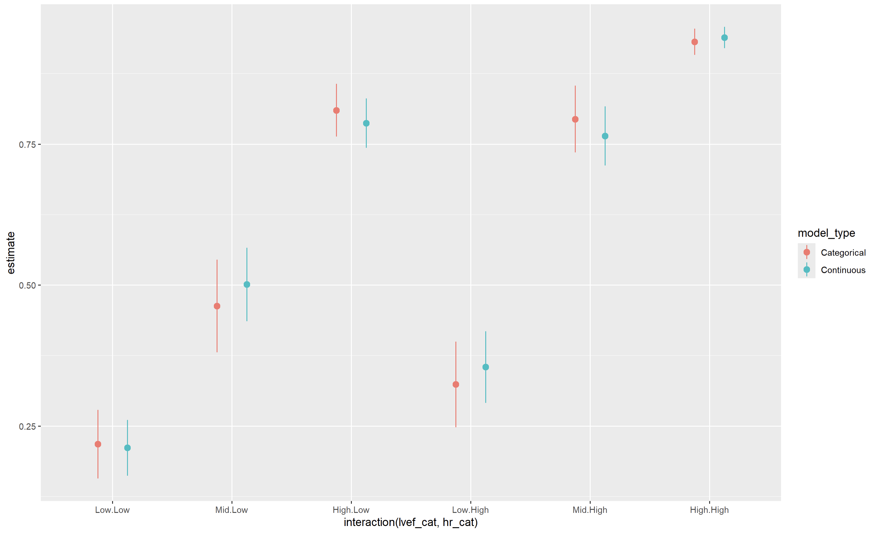
The point estimates are reasonably similar between both models, though standard errors/CIs are smaller for the continuous model (as would be expected).
Would love to hear some feedback/criticism of this approach. Some flaws I’ve thought of:
1. As with a pre-categorized model, you’re hiding some heterogeneity within each of these strata.
2. When interpreting the the joint effect of 2 predictors (here LVEF and HR), the picture is somewhat muddled since the distribution of LVEF may not be the same in the group with a low versus high heart rate (So the “Low EF.Low HR” and the “Low EF.High HR” estimates don’t exactly isolate the effect of HR). Again, this is also inherent to the categorized model.
3. You may have to expend a few more lines in the Methodology section explaining what you did.
4. Computationally more demanding than a pre-categorized model (since you’d be marginalizing over several predictions rather than making a single prediction for the desired category), particularly with very large datasets where you’d marginalize over very many rows. A potential solution in that case would be to take a random sample of your dataset and marginalize over that.
Other than 3. and 4., is there any clear disadvantage of this approach compared to using a pre-categorized model? (the disadvantages versus a continuous approach are clearcut)
*Some would argue that the “Low/Mid/High” marginalized predictions in the above plot could just be replaced with conditional predictions at (for example), the first, second, and third quartiles. I agree and have done this before, but often a common query would be “What do you mean the risk corresponds to an EF of exactly 35% or 65%? Don’t you mean <35% or >65%?”
To be clear, this is not a substitute for full continuous displays (which should be provided), but is merely intended as a less-damaging substitute to the full use of pre-categorized models.