What is the optimal way to combine multiple imputation and bootstrap to quantify uncertainty in discrimination and calibration metrics for the internal validation of diagnostic or prognostic models?
I am constructing a proportional odds logistic model for the purpose of predicting prognosis of Covid-19 at the time of first contact with the healthcare system (see preprint here). The model is derived on prospectively collected data on roughly 4.500 consecutively diagnosed SARS-CoV-2 positive patients in Iceland.
There are some missing data. I aim to combine multiple imputation (MI) with bootstrapping to report confidence intervals around discrimination and calibration measures of the fitted model. Several simulation studies have shown that some combinations of MI and bootstrap may yield asymptotically biased results and incorrect nominal coverage of the confidence intervals under differing circumstances, see Bartlett & Hughes, Schomaker & Heumann and Wahl et al.
My aim is to understand these papers in more detail and specifically how they would apply to my problem using aregImpute() and fit.mult.impute() from the Hmisc package.
As far as I can tell, the linked papers above (with slight variations) describe three combinations of MI and bootstrap, which they then compare. The Bartlett & Hughes paper summarises these three approaches so well that any attempt of mine to restate them would not do them justice. In the words of Bartlett and Hughes, the three approaches are
-
Multiple imputation and then bootstrap to estimate the within-imputation complete data variance:
-
Multiple imputation followed by a pooled percentile of bootstrap resamples with replacement
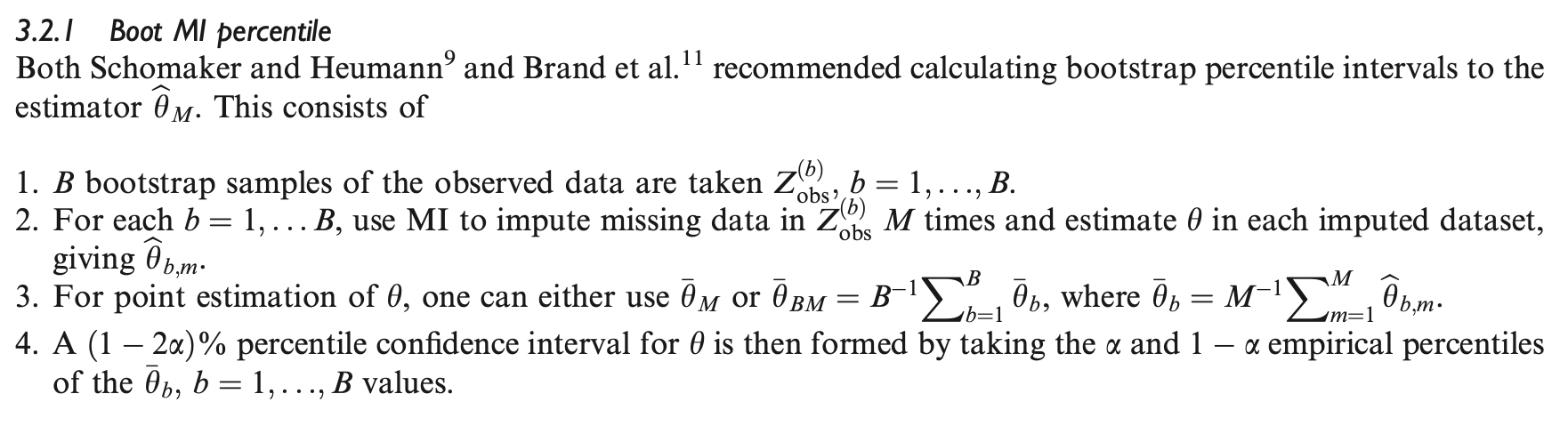

- Bootstrap from the observed data and then apply MI to each bootstrap sample with replacement, then taking a pooled percentile.

Bartlett and Hughes find that only 3) Boot MI percentile approach will provide nominal coverage under uncongeniality or misspecification of the imputation and analysis procedures. If I have misunderstood or mischaracterised the problem, I would appreciate any and all corrections or suggestions for further reading.
Now to the question. I have trouble understanding exactly how aregImpute() performs its multiple imputation and how it fits into the above classification. The way I understand it, aregImpute() first takes bootstraps with replacement from the observations in the entire dataset and the fits the multiple imputation model on the bootstrap sample. It then imputes the missing value of the target variable by finding a non-missing observed value in the entire dataset using complex weighting, and imputing this value. It seems to me this most closely matches to 3) Boot MI, where M = 1, i.e. only one imputation is performed for each bootstrap resample.
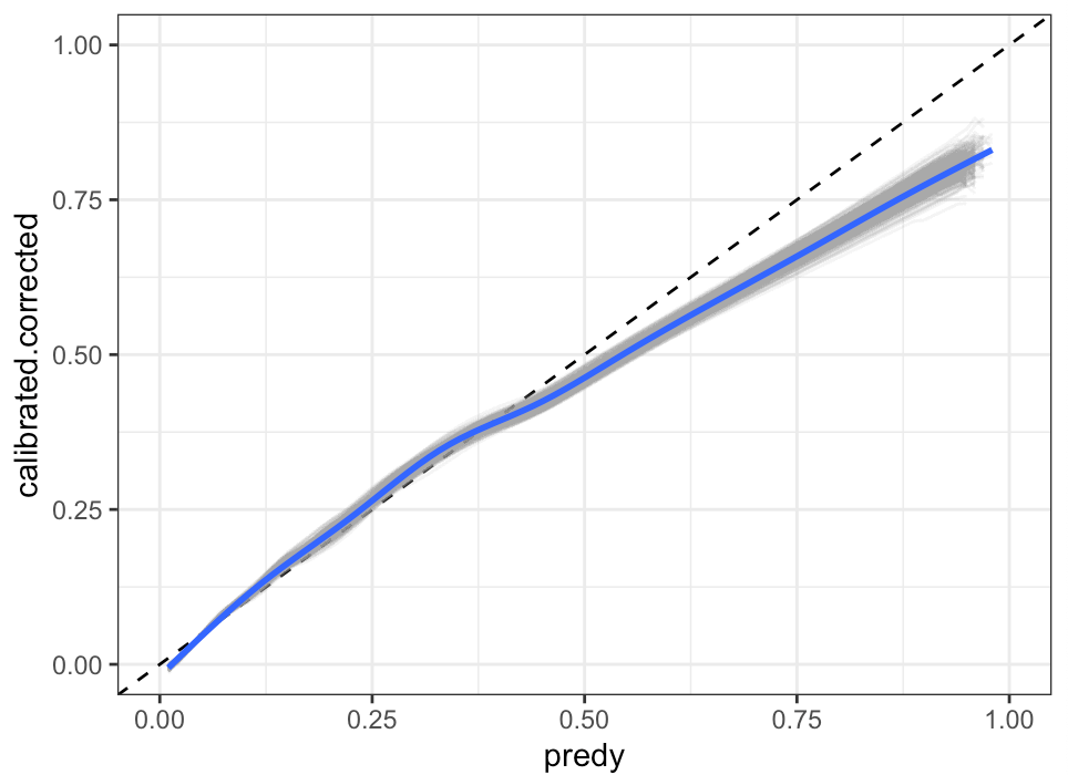
The problem arises when I would like to construct a confidence interval around discrimination metrics (such as the C-statistic). calibration metrics (calibration intercept, calibration slope), and most importantly, confidence intervals around the non-parametric calibration curve between observed and predicted risk. In the pre-print, I followed my interpretation of the general recommendations in Regression modelling strategies and Clinical Prediction Models: A Practical Approach to Development, Validation, and Updating, to take a randomly selected singly imputed dataset and repeatedly fit the model to bootstrap resamples with replacement of the singly imputed dataset. I do this 2000 times and construct the confidence intervals using a percentile based approach. During review it was pointed out to me that this approach does not include any of the between-imputation uncertainty.
I can think of two ways to resolve this but I am unsure if they 1) are valid and 2) if they are compatible with any of the general approaches described by the above papers.
The first solution would be to iterate the process at the level of aregImpute(), such that for each step in the iteration process, I would constructed M = 5 imputed datasets, apply fit.mult.impute() to apply the proportional odds regression model to obtain the relevant statistics that are average over the 5 imputed datasets, and extract the relevant statistic. I would repeat this 1000 times and construct a percentile based confidence interval [alpha, 1 - alpha]. This would be enormously computationally expensive as I would have to construct 5000 imputed datasets by fitting 1000 imputation models and then fit an analysis model 1000 times. This seems excessive.
The second solution which I am more happy with would be to iterate over a random draw of singly imputed datasets. First I would run aregImpute() producing M = 100 imputed datasets. Then I would iterate such that for each iteration, a randomly selected singly imputed dataset is selected, and the proportional odds regression model applied to a bootstrap resample with replacement from the selected dataset. Finally, the relevant statistic would be extracted. This would be repeated 1000 times and a percentile based confidence interval would be constructed. This would be less computationally expensive but comes with the drawback of the fitted models ignoring the imputation-corrected variance-covariance matrix.