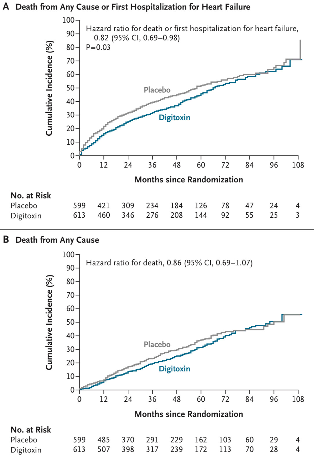
Hey there, I am an interventional cardiologist with special interest in heart failure and there was recently published the DIGIT-HF Trial in the NEJM (pdf online here) When I read the study I was kind of irritated, why the visually seeable heterogeneity of the hazards in time was not addressed in any detail. Probably I am missing something, but when I look at the Kaplan-Meier curves Figure 1 A-C (see also below), I am not convinced, that the proportional hazard assumption holds, and this would directly effect the statement, that the Digitoxin effect is really significant. If one would landmark at 48 months, the effect would be reversed, wouldn‘t it?
Maybe some of you statistical and methodological experts can enlighten me, how this visible effect is incorporated into the statistical aspects especially in the analysis of the primary endpoint.
Thank you for any input and helping me understand this study.
This is a great question Chris, and I hope that others will add their thoughts. Here are mine, in no particular order.
Clinical trialists have done a poor job of eliciting patient utilities that can tell us how to weight various outcomes and time frames.
Without utilities you can’t tell for sure which treatment is preferred. If a utility function puts all the weight on the last follow-up time, there is no evidence for benefit, as you said. If the utility function is more like expected months event-free, then the Cox model analysis is likely to concur with a finding that we expect patients on dig to expect to spend more time alive.
If the incidence curves or the HR are not covariate adjusted, we should ignore them until we get valid adjusted estimates. This is not for imbalances but to account for within-treatment outcome heterogeneity. Kaplan-Meier estimates are intended only to apply to homogeneous samples.
Incidence curves should not be presented without confidence bands for the difference in incidence.
Statisticians get a grade of F for insisting that all key analyses have only one parameter for treatment. We should routinely expect non-proportional hazards, and so we should routinely model things such as treatment \times \log(t) interaction. Then we estimate, with confidence bands, treatment effect as a function of time. This kind of relaxed model also should form the basis for estimating restricted mean survival time, not homogeneity-assuming Kaplan-Meier estimates. This is an exact analogy to the classic two-sample problem for continuous Y where if using a t-test we should routinely allow for unequal variances in the treatment groups.
A great overall test for a difference in adjusted survival curves would be the 2 d.f. test that comes from jointly testing the treatment coefficient and the \log(t) interaction with treatment coefficient. This is described here.
Hopefully I haven’t misunderstood the question. Basically, the proportional hazards assumption can only hold if there are no effects (see https://doi.org/10.1093/aje/kwae361). There has been some interesting research initiated by Miquel Hernan in 2010 (DOI: 10.1097/EDE.0b013e3181c1ea43). Here’s another good reference: doi:10.1001/jama.2020.1267, and a more technical one: Subtleties in the interpretation of hazard contrasts | Lifetime Data Analysis .
I guess the incidence curves would cross if there were a treatment effect. Then the frail would die first in the non-treatment group, leaving the robust alive, while in the treatment group the frail would be kept alive initially.
Even without knowing this literature above, I don’t think the proportional hazards assumption is needed when comparing Kaplan-Meier curves based on stratified data? I assume the idea is to estimate the probability from time zero, but I’m not sure about the purpose of a landmark at 48 months? -maybe I’m missing something?
Right, K-M estimates are nonparametric, just assuming independence of censoring and event risk. But they assume homogeneity of outcomes since they are not covariate adjustment. Such homogeneity is almost impossible.
My thought was, if one would cut the time into two sections, the first 48 months and then after the 48 months. In the first 48 months there would be a clear benefit. In the months after month 48, one can restart the survival curves at the same level and Digitoxin would have a much higher event rate.
Interesting literature, didnt knew this beforehand.
I get your point with crossing curves, but I would assume, that at the point the frail people die in the treatment group there would be “new” frail people in the non-treatment group due to time is going on. And thats why one always see this effect of kind of parallel curves in RCTs in the long run, isnt it?
My gut feeling is, that it’s kinda misleading, if one shows that in the long run the medication has no effect (by showing this long follow-up), but the idea was to show a benefit in the short run.
Shouldn’t the endpoint then be “mean-survival-time” instead of mortality at longest follow-up?
Very good points. I was often thinking, why CI’s are not shown in so many trials, it would visually help a lot.
Maybe it is a clinician and statistical/programming newbie question, but do there exist something like “covariate adjusted Kaplan-Meier-curves”? I normally use rms, cph and ggsurvplot for my survival plots, but never thought, if there would be a more appropriate visual representation which corresponds to the multivariable model results.
Really good comparison, in the t-test setting it gets accepted more and more but the survival setting is pushed aside to the methods “we did this always, so it has to be right”.
Do you have a literature hint, where such a modelling is described in more detail (maybe with code examples)?
The paper from Bredlow, Esler and Berger is really tough stuff for a non-mathematician, but I got the idea behind it and this is exactly the situation for the in the original post shown KMs!
At time zero/baseline, when individuals were randomized, each person had the same chance of receiving digitoxin or placebo - ie the individuals were statistically exchangeable at baseline. If digitoxin lowers the incidence of death, then after 48 months they are no longer exchangeable (some frail individuals in the digitoxin group have survived, while some frail individuals in the placebo group have died). Thus, they are no longer randomized to digitoxin after time 0 - eg at time 48 months.
One cannot condition on surviving 48 months and restart the analysis, because we cannot know at time zero who will survive. Of course, with the data in hand we do know who survived - but that is the mortal sin of conditioning on the future. Probably @f2harrell wouldn’t even give an F for conditioning on the future
I understand it correctly, i disagree with the statement: “And that’s why one always sees this effect of kind of parallel curves in RCTs in the long run, isn’t it?” Rather, the lines cannot be parallel if the treatment is lower the risk of dying early. It might appear that they are parallel - either by lack of power to see they are not or because a reviewer asks us to test for proportional hazards. But they cannot truly be parallel and show an effect at the same time (see modification/details in the papers mentioned above). This is why we add log(t) × treatment, and why @f2harrell gives an F to those who dont
Good point about looking at mean survival time. At 108 months (9 years), only 4 individuals remain at risk in both groups, and most have died or been censored. This may suggest they were quite old at baseline (or that it was a very deadly disorder, I didn’t look at the paper). Eg if they were around 80 at baseline, most would be expected to die within 9 years anyway. Thus no medication can prevent death in the long run, although some can lower the risk in the short run. The mean-survival-time may show the digitoxin group have longer life expectancy at baseline but they are all dead (expect 4) after 9 years
This is as simple as stratifying on treatment but covariate-modeling everything else. The only hard part is deciding which covariate settings to display. There is an example in 20 Cox Proportional Hazards Regression Model – Regression Modeling Strategies . I think I default to setting all covariates to median/mode but that could really be debated.
I struggle with this. I think for a lot of cases you can rightly emphasize mean covariate-specific survival time, giving credit to a treatment that delays death even if at 5 years the cumulative incidence is the same as control. A clear choice where you only care where you end up is weight loss studies. A clear example where “how you got there” matters is pain studies, where if a treatment can give a patient a year with minimal pain we would view that as a “win” even if pain reappeared later.
All KM all cause death curves must eventually converge because everyone dies. Therefore we can’t expect to observe parallel curves (thanks @Frank for telling us to ignore them). The greater the mortality the more likely we are to observe converging curves - this study has high mortality so no surprise seeing them converge.
Well put, still leaving the questions of which summary measures to emphasize when the follow-up is, say, 2-10y. A great research project would involve eliciting from a large number of patients or normal volunteers (which?) their preferences for decision making from among choices such as
cumulative incidence at t years for various values of t